Cylindrical Pressure Vessel

A long cylindrical thick walled pressure vessel is here subjected to both a high internal pressure and thermal expansion. The model and solution is symmetric and also suitable for modeling with the two-dimensional plane strain approximation. This problem allows for an analytical solution which is used to validate and test the accuracy of the simulation [1].

Tutorial

This model is available as an automated tutorial by selecting Model Examples and Tutorials... > Structural Mechanics > Cylindrical Pressure Vessel from the File menu. Or alternatively, follow the step-by-step instructions below.

1. To start a new model click the New Model toolbar button, or select New Model... from the File menu.
2. Select the 2D radio button.
3. Select the Plane Strain physics mode from the Select Physics drop-down menu.
4. Press OK to finish the physics mode selection.

To decrease the time and cost of the simulation, symmetry and and the plane strain approximation are used so that only a quarter of a 2D slice has to be modeled.

The geometry can be created by first subtracting a smaller inner from a larger outer cylinder. And the overlaying a rectangle and using the intersection operation to get the resulting quarter geometry section.

1. To create a circle or ellipse, first click on the Create circle/ellipse Toolbar button. Then left click in the main plot axes window, and hold down the mouse button. Move the mouse pointer to draw the shape outline, and release the button to finalize the shape.
2. Select E1 in the geometry object Selection list box.
3. To modify and edit the selected ellipse, click on the Inspect/edit selected geometry object Toolbar button to open the Edit Geometry Object dialog box.
4. Enter 0 0 into the center edit field.
5. Enter 0.95 into the x_radius edit field.
6. Enter 0.95 into the y_radius edit field.
7. Press OK to finish and close the dialog box.
8. To create a circle or ellipse, first click on the Create circle/ellipse Toolbar button. Then left click in the main plot axes window, and hold down the mouse button. Move the mouse pointer to draw the shape outline, and release the button to finalize the shape.
9. Select E2 in the geometry object Selection list box.
10. To modify and edit the selected ellipse, click on the Inspect/edit selected geometry object Toolbar button to open the Edit Geometry Object dialog box.
11. Enter 0 0 into the center edit field.
12. Enter 0.2 into the x_radius edit field.
13. Enter 0.2 into the y_radius edit field.
14. Press OK to finish and close the dialog box.
15. Select E1 and E2 in the geometry object Selection list box.
16. Press the - / Subtract geometry objects Toolbar button.
17. To create a rectangle, first click on the Create square/rectangle Toolbar button. Then left click in the main plot axes window, and hold down the mouse button. Move the mouse pointer to draw the shape outline, and release the button to finalize the shape.
18. Select R1 in the geometry object Selection list box.
19. To modify and edit the selected rectangle, click on the Inspect/edit selected geometry object Toolbar button to open the Edit Geometry Object dialog box.
20. Enter 0 into the x_min edit field.
21. Enter 1 into the x_max edit field.
22. Enter 0 into the y_min edit field.
23. Enter 1 into the y_max edit field.
24. Press OK to finish and close the dialog box.
25. Select CS1 and R1 in the geometry object Selection list box.
26. Press the & / Intersect geometry objects Toolbar button.
27. Switch to Grid mode by clicking on the corresponding Mode Toolbar button.
28. Enter 0.02 into the Grid Size edit field.
29. Press the Generate button to call the grid generation algorithm.
30. Switch to Equation mode by clicking on the corresponding Mode Toolbar button.
31. Equation and material coefficients can be specified in Equation/Subdomain mode. In the Equation Settings dialog box, enter 0.33 for the Poisson's ratio and 2e11 for the Modulus of elasticity, 1.3e-5 for the Thermal expansion coefficient, and the expanded expression for the temperature field (Ti-To)/log(ro/ri)*log(ro/r)+To. The other coefficients can be left to their default values.
32. Enter (600-30)/log(0.95/0.2)*log(0.95/sqrt(x^2+y^2))+30 into the Temperature edit field.
33. Press OK to finish the equation and subdomain settings specification.
34. Switch to Boundary mode by clicking on the corresponding Mode Toolbar button.

To account for the symmetry, fix the x-displacement of the left vertical boundary by setting the displacement in the x-direction there to zero, and similarly fix the y-displacement on the lower horizontal boundary.

1. Select 3 in the Boundaries list box.
2. Select the Fixed displacement, v radio button.
3. Select 4 in the Boundaries list box.
4. Select the Fixed displacement, u radio button.

Apply the normal pressure 6e7 on the inner boundary and 2.5e7 on the outer one. Note that these loads are scaled with the outward pointing unit normal vectors nx and ny in order to apply the forces normal to the boundaries.

1. Select 2 in the Boundaries list box.
2. Enter -nx*6e7 into the Displacement/load, x-component edit field.
3. Enter -ny*6e7 into the Displacement/load, y-component edit field.
4. Select 1 in the Boundaries list box.
5. Enter -nx*2.5e7 into the Displacement/load, x-component edit field.
6. Enter -ny*2.5e7 into the Displacement/load, y-component edit field.
7. Press OK to finish the boundary condition specification.
8. Switch to Solve mode by clicking on the corresponding Mode Toolbar button.
9. Press the = Toolbar button to call the solver. After the problem has been solved FEATool will automatically switch to postprocessing mode and plot the computed solution.

The analytical solution for the displacement and stresses in the radial direction are as follows

	r = 0.2	r = 0.95
r-displacement	0.00068	0.00302
r-stress	-6e7	-2.5e7
th-stress	-1.59e9	0.59e9
z-stress	-2.1e9	0.107e9

1. Press the Plot Options Toolbar button.
2. Select Stress, x-component from the Predefined surface plot expressions drop-down menu.
3. Press OK to plot and visualize the selected postprocessing options.

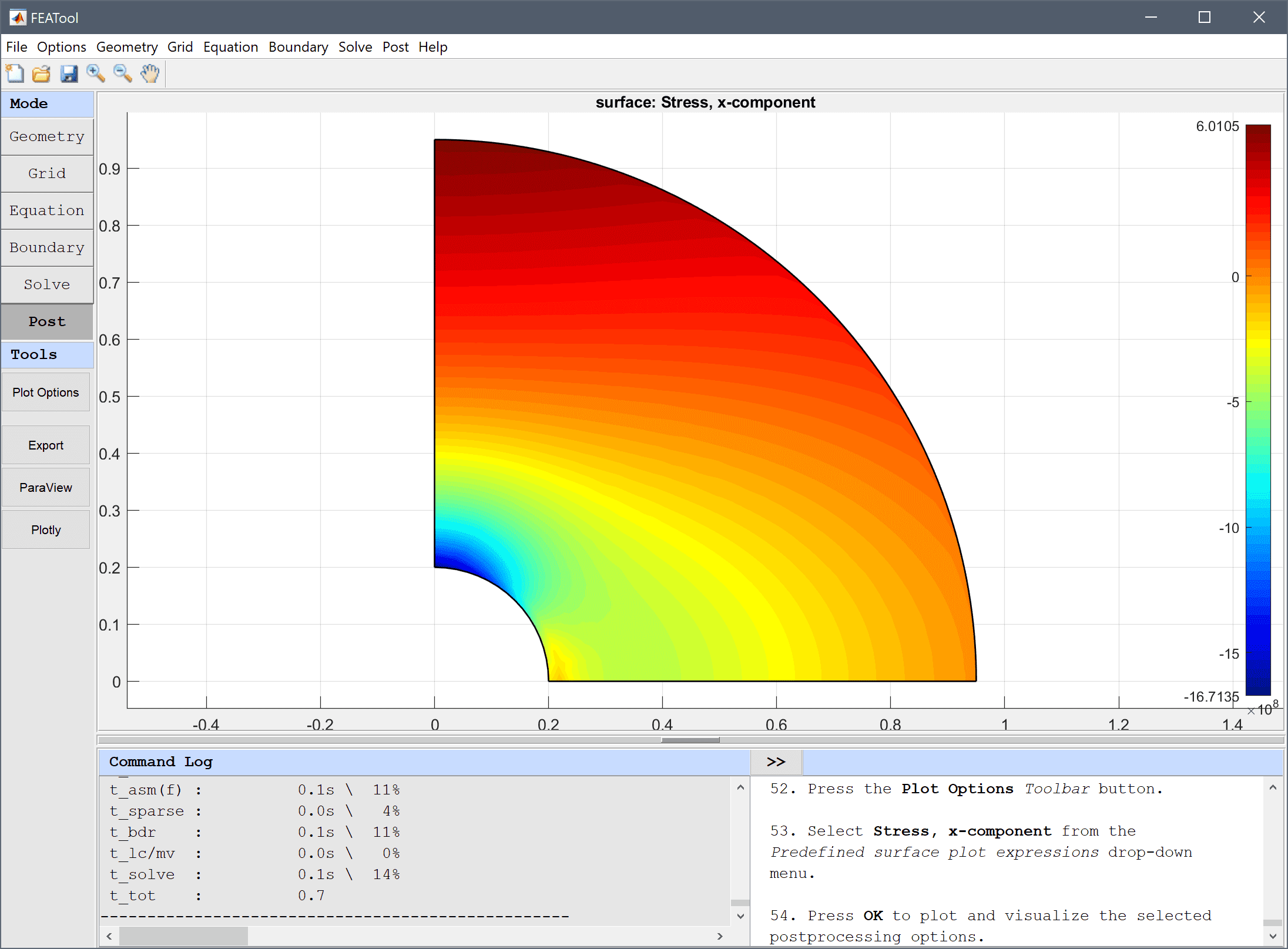
To compare it is easier to either look at the horizontal x-axis (where the x-direction quantities correspond to the radial ones) or alternatively the vertical y-axis. Click anywhere on the surface plot to evaluate the expression in the chosen point. For a more clear representation one can use the Point/Line Evaluation functionality to study and plot quantities at points and lines.

1. Select Point/Line Evaluation... from the Post menu.
2. Select x-displacement from the Evaluation Expression drop-down menu.
3. Enter 0.2:0.01:0.95 into the Evaluation coordinates in x-direction edit field.
4. Enter 0 into the Evaluation coordinates in y-direction edit field.
5. Press OK to finish and close the dialog box.

The cylindrical pressure vessel structural mechanics model has now been completed and can be saved as a binary (.fea) model file, or exported as a programmable MATLAB m-script text file (available as the example ex_planestrain2 script file), or GUI script (.fes) file.

Reference

[1] Barber JR. Solid Mechanics and Its Applications, Intermediate Mechanics of Materials. vol. 175, 2nd ed. Springer, 2011.