|
|
FEATool Multiphysics
v1.18.1
Finite Element Analysis Toolbox
|
|
|
FEATool Multiphysics
v1.18.1
Finite Element Analysis Toolbox
|
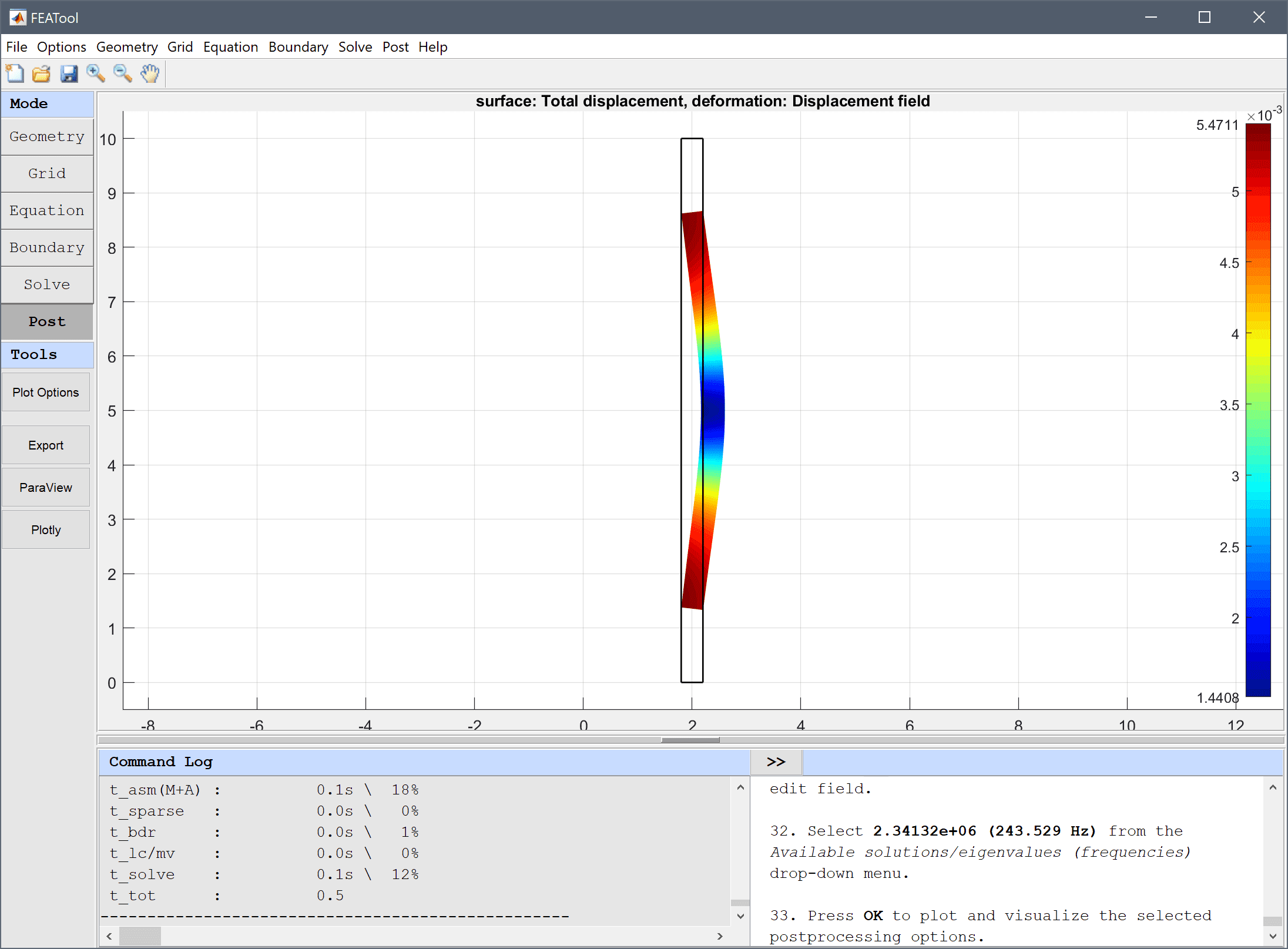
This model studies the vibration modes of a free and hollow cylinder using an axisymmetric approximation. No loads or constrains are applied as the free modes are sought. The cylinder is 10 m long, has a center diameter of 2 m, and is 0.4 m thick. Moreover, the material of the cylinder is considered to be steel with E = 2·1011 Pa, density 8000 km/m3, and a Poisson's ratio of 0.3. Target free vibration frequencies are given in [1].
This model is available as an automated tutorial by selecting Model Examples and Tutorials... > Structural Mechanics > Vibration Modes of a Hollow Cylinder from the File menu. Or alternatively, follow the step-by-step instructions below.
1.8 into the xmin edit field.2.2 into the xmax edit field.0 into the ymin edit field.10 into the ymax edit field.0.2 into the Grid Size edit field.0.3 into the Poisson's ratio ν edit field.2e11 into the Modulus of elasticity E edit field.8000 into the Density ρ edit field.Open the postprocessing settings dialog box, look at the Solution eigenvalue/frequency drop-menu box, and verify that they correspond to the target values 0, 243.8, 378.5, 394, 397.5, 405 Hz. Select the second mode and plot its Total displacement as well as Deformation plot with a scale factor of 1.
0.2 into the Deformation scale factor edit field.The vibration modes of a hollow cylinder structural mechanics model has now been completed and can be saved as a binary (.fea) model file, or exported as a programmable MATLAB m-script text file (available as the example ex_axistressstrain1 script file), or GUI script (.fes) file.
To visualize the full 3D solution from the axisymmetic model, the data can be exported and processed on the MATLAB command line interface (CLI) console with the Export Model Data Struct to MATLAB option from the File menu. The postrevolve and postplot functions can then be applied to revolve and visualize the data, for example
fea_revolved = postrevolve( fea, 36, 1 );

% Note that the radial coordinate is replaced by
% "x" and "y" in the revolved 3D fea data struct
postplot( fea_revolved, 'surfexpr', 'sqrt((sqrt(x^2+y^2)*u)^2+w^2)', ...
          'deformexpr', {'x*u', 'y*u', '0'}, 'deformscale', -0.2, ...
          'solnum', 4, 'parent', figure, 'axis', 'off', 'colorbar', 'off' )
view(3)
[1] Abbassian F, Dawswell DJ, Knowles NC. Free Vibration Benchmarks. NAFEMS, Test 41, 1987.