FEATool Multiphysics  v1.16.5
Finite Element Analysis Toolbox
Stress Analysis of a Thick Plate

This is a benchmark and validation model for linear elasticity where an elliptical thick plate with a hole is subjected to a uniform pressure load of 106 MPa [1]. The outer surface is assumed to be constrained from expansion, in addition to the center line which is fixed in the z-direction. Symmetry is also utilized so that only a quarter of the geometry is modeled.

Tutorial

This model is available as an automated tutorial by selecting Model Examples and Tutorials... > Structural Mechanics > Stress Analysis of a Thick Plate from the File menu. Or alternatively, follow the step-by-step instructions below.

  1. To start a new model click the New Model toolbar button, or select New Model... from the File menu.
  2. Select the 3D radio button.
  3. Select the Linear Elasticity physics mode from the Select Physics drop-down menu.
  4. Press OK to finish the physics mode selection.

The elliptical shape can be constructed by first making two elliptical cylinders and subtracting the smaller inner one from the outer larger one.

  1. Press the Create cylinder Toolbar button.
  2. Enter 0 0 0 into the center edit field.
  3. Enter 0.3 into the length edit field.
  4. Enter 3 into the axis edit field.

Approximation of curved boundaries can be improved by increasing the polygon resolution of the geometry object. This however will lead to an increased time and cost for performing geometry object operations.

  1. Enter 32 into the resolution edit field.
  2. Press OK to finish and close the dialog box.

An elliptical cylinder is easiest to create by scaling the unit cylinder.

  1. Select C1 in the geometry object Selection list box.
  2. Press the Copy and/or transform selected geometry object Toolbar button.
  3. Enter 2 1 1 into the Space separated string of coordinate scaling factors edit field.
  4. Press OK to finish and close the dialog box.
  5. Press the Create cylinder Toolbar button.
  6. Enter 0 0 0 into the center edit field.
  7. Enter 0.3 into the length edit field.
  8. Enter 3 into the axis edit field.
  9. Enter 32 into the resolution edit field.
  10. Press OK to finish and close the dialog box.
  11. Select C2 in the geometry object Selection list box.
  12. Press the Copy and/or transform selected geometry object Toolbar button.
  13. Enter 3.25 2.75 1 into the Space separated string of coordinate scaling factors edit field.
  14. Press OK to finish and close the dialog box.

To decrease the time and cost of the simulation, symmetry is utilized so that only a quarter of the geometry has to be modeled. To do this create a block overlapping one of the quarters, the use the Intersect tool to keep the overlapping objects.

  1. Press the Create cube/block Toolbar button.
  2. Enter 3.5 into the xmax edit field.
  3. Enter 3 into the ymax edit field.
  4. Enter -0.1 into the zmin edit field.
  5. Enter 0.5 into the zmax edit field.
  6. Press OK to finish and close the dialog box.

Subtract the outer from inner cylinder, while intersecting the resulting object with the block. Note that the edges and dimensions of the inner cylinder and block are larger than required instead of parallel and in-line, for more robust geometry operations.

  1. Select Combine Objects... from the Geometry menu.
  2. Enter TF2 - TF1 & B1 into the Geometry Formula edit field.
  3. Press OK to finish and close the dialog box.
  4. Select CI1 in the geometry object Selection list box.

In order to create edges at z = 0, on which to impose boundary conditions, two parallel objects can be created by copying the first and offsetting it to the lower half plane.

  1. Select Copy/Transform Object... from the Geometry menu.
  2. Select the Make copy of geometry object check box.
  3. Enter 0 0 -0.3 into the Space separated string of displacement lengths edit field.
  4. Press OK to finish and close the dialog box.
  5. Switch to Grid mode by clicking on the corresponding Mode Toolbar button.
  6. Press the Settings Toolbar button.
  7. Enter 0.1 into the Subdomain Grid Size edit field.
  8. Press the Generate button to call the grid generation algorithm.
  9. Press OK to finish and close the dialog box.
  10. Switch to Equation mode by clicking on the corresponding Mode Toolbar button.
  11. Select both subdomains in the Equation Settings dialog box and enter 0.3 for the Poisson's ratio and 2.1e11 for the Modulus of elasticity.
  12. Press OK to finish the equation and subdomain settings specification.
  13. Switch to Boundary mode by clicking on the corresponding Mode Toolbar button.
  14. Select the top boundary (number 4) and enter the -1e6 for the load force in the negative z-direction.

Also fix the x and y displacements on the outer boundaries.

  1. Select 1 and 6 in the Boundaries list box.
  2. Select the Fixed displacement, u radio button.
  3. Select the Fixed displacement, v radio button.

Due to the symmetry the x-displacement should be fixed on boundaries 3 and 8.

  1. Select 3 and 8 in the Boundaries list box.
  2. Select the Fixed displacement, u radio button.

And similarly the y-displacement should be fixed on boundaries 2 and 7.

  1. Select 2 and 7 in the Boundaries list box.
  2. Select the Fixed displacement, v radio button.
  3. Press OK to finish the boundary condition specification.
  4. Select Add Edge Constraints... from the Boundary menu, and add the constraint w = 0 to fix the displacement in the z-direction of the outer horizontal edge at z = 0 (number 4).
  5. Switch to Solve mode by clicking on the corresponding Mode Toolbar button.
  6. Press the = Toolbar button to call the solver. After the problem has been solved FEATool will automatically switch to postprocessing mode and plot the computed solution.
  7. From the reference the stress in the y-direction at the inner point p = (2, 0, 0.3) should be -5.38 MPa. One can use the Plot Options to plot the y-component stress to visually confirm the solution.
  8. Press the Plot Options Toolbar button.
  9. Select the Surface Plot check box.
  10. Select Stress, y-component from the Predefined surface plot expressions drop-down menu.
  11. Press OK to plot and visualize the selected postprocessing options.
  12. Alternatively, the Point/Line Evaluation functionality can be used to evaluate and extract numeric values in specific points and on lines.
  13. Select Point/Line Evaluation... from the Post menu.
  14. Select Stress, y-component from the Evaluation Expression drop-down menu.

Note that a small offset, such as +/-sqrt(eps) can sometimes be required to ensure the evaluation points are inside the domain.

  1. Enter 
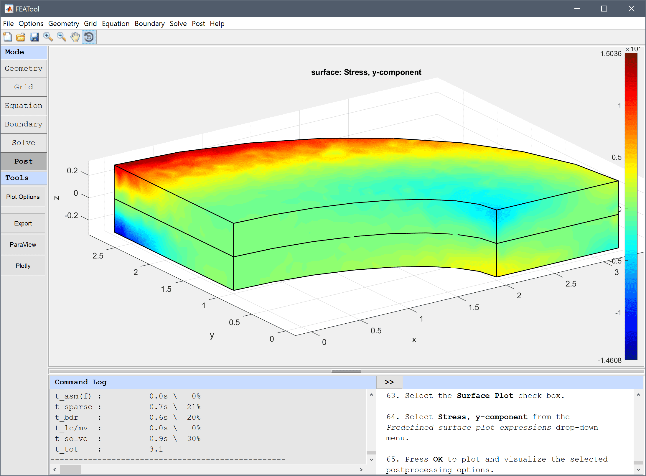
2 into the Evaluation coordinates in x-direction edit field.
  2. Enter 0 into the Evaluation coordinates in y-direction edit field.
  3. Enter 0.3 into the Evaluation coordinates in z-direction edit field.
  4. Press the Apply button.
  5. Press OK to finish and close the dialog box.

The stress analysis of a thick plate structural mechanics model has now been completed and can be saved as a binary (.fea) model file, or exported as a programmable MATLAB m-script text file, or GUI script (.fes) file.

Reference

[1] Davies G, Fenner RT, Lewis RW. NAFEMS Background To Benchmarks. LE10 Thick plate - normal pressure, 1992.