Temperature Loading of a Tapered Cylinder

This validation test case models temperature loading of a tapered hollow thick cylinder with a spherical bottom flange section. The solid object is assumed to be clamped vertically, but allowed to expand horizontally due to a linear temperature gradient. The stress in the z-direction at the bottom inner point is computed and compared to a reference value [1].

Tutorial

This model is available as an automated tutorial by selecting Model Examples and Tutorials... > Structural Mechanics > Temperature Loading of a Tapered Cylinder from the File menu, viewed as a video tutorial, or alternatively, follow the step-by-step instructions below.

1. To start a new model click the New Model toolbar button, or select New Model... from the File menu.
2. Select the 3D radio button.

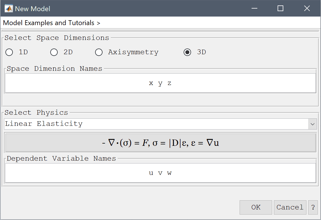
3. Select the Linear Elasticity physics mode from the Select Physics drop-down menu.

   
4. Press OK to finish the physics mode selection.

The geometry consists of a thick cylindrical pipe section connected to a spherical bottom flange with a taper. As the geometry is axially symmetric, it is easiest to create by first using a 2D workplane to draft the cross-section, which then can be revolved into the three dimensional space.

1. Select 2D Workplane... from the Geometry menu.

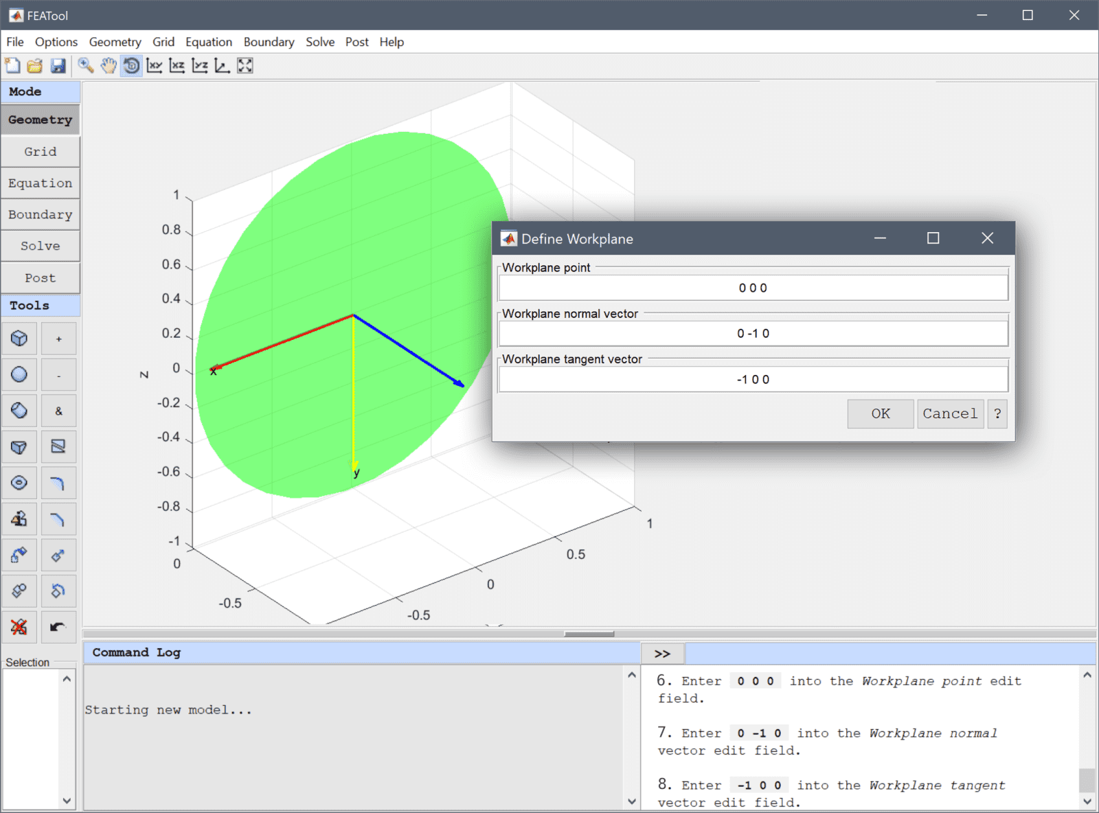
Workplanes are defined by a point (local origin), normal (blue) and tangent vectors (yellow and red). The green circle shows a preview where the plane will be located in 3D space.

1. Enter 0 0 0 into the Workplane point edit field.
2. Enter 0 -1 0 into the Workplane normal vector edit field.

3. Enter -1 0 0 into the Workplane tangent vector edit field.

   

Note that the local coordinate system will be mirrored in the y-axis. The outline sketch will therefore be drawn upside down so as to be in the positive half-plane of the 3D space.

1. Press OK to finish and close the dialog box.

First create a rectangle to cover the modeling region.

1. Select Rectangle from the Geometry menu.
2. Enter 0.7071 into the x_min edit field.
3. Enter 1.4 into the x_max edit field.
4. Enter -1.79 into the y_min edit field.
5. Enter 0 into the y_max edit field.
6. Press OK to finish and close the dialog box.

Now create two circles, one with radius 1 and the other with 1.4.

1. Select Circle from the Geometry menu.
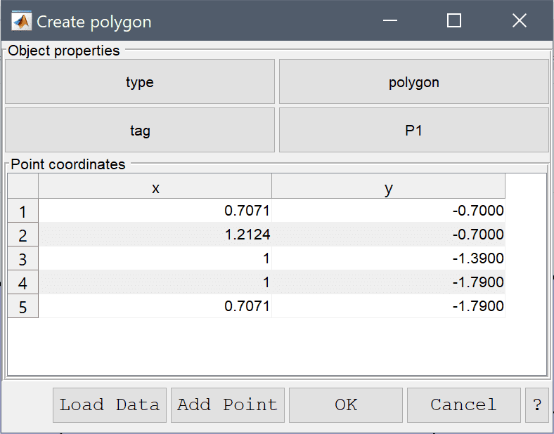
2. Enter 1 into the radius edit field.
3. Press OK to finish and close the dialog box.
4. Select Circle from the Geometry menu.
5. Enter 1.4 into the radius edit field.
6. Press OK to finish and close the dialog box.

Then make a polygon for the cylindrical connection.

1. Select Polygon from the Geometry menu.

Enter the following data into the Point coordinates table.

	x	y
1	0.7071	-0.7
2	1.2124	-0.7
3	1	-1.39
4	1	-1.79
5	0.7071	-1.79

1. Press OK to finish and close the dialog box.

The shape of the cross-section can be created by joining the polygon with the outer circle, subtracting the inner circle, and taking the intersection with the rectangle.

1. Select C2 and P1 in the geometry object Selection list box.

   
2. Press the + button.
3. Select CJ1 and C1 in the geometry object Selection list box.
4. Press the - button.
5. Select R1 and CS1 in the geometry object Selection list box.

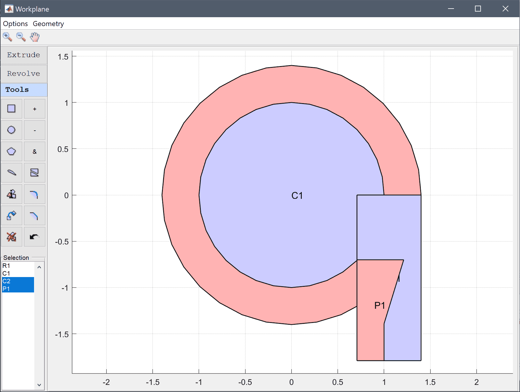
6. Press the & button.

   

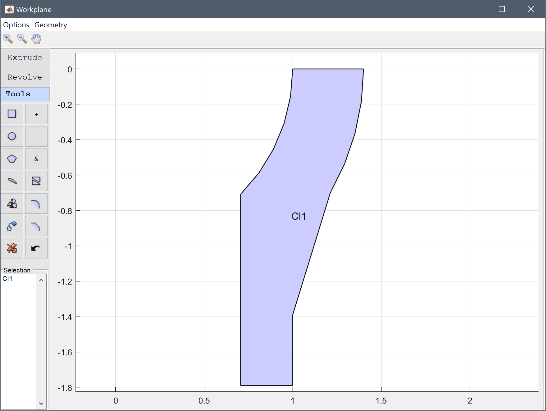
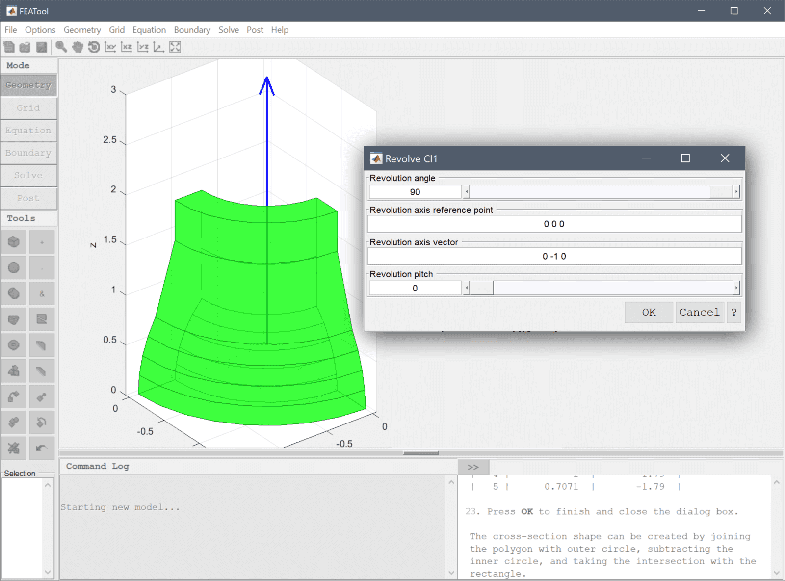
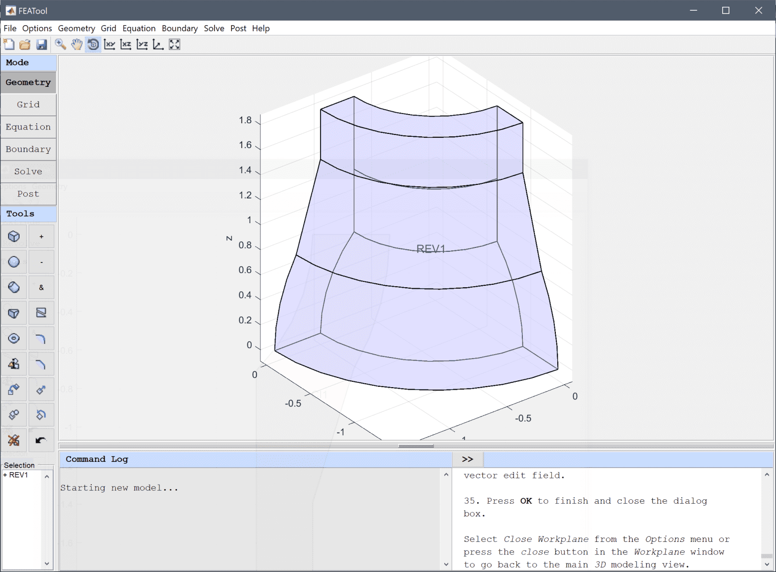
The 2D outline sketch can now be revolved to a 3D solid (an outline preview of the revolution shape is shown in the 3D view). As this geometry is symmetric it is enough to model a quarter section and thereby also reducing the mesh size leading to faster simulations.

1. Select CI1 in the geometry object Selection list box.
2. Press the Revolve button.
3. Enter 90 into the Revolution angle edit field.
4. Enter 0 0 0 into the Revolution axis reference point edit field.

5. Enter 0 -1 0 into the Revolution axis vector edit field.

   
6. Press OK to finish and close the dialog box.

Select Close Workplane from the Options menu or press the close button in the Workplane window to go back to the main 3D modeling view.

1. Switch to Grid mode by clicking on the corresponding Mode Toolbar button.

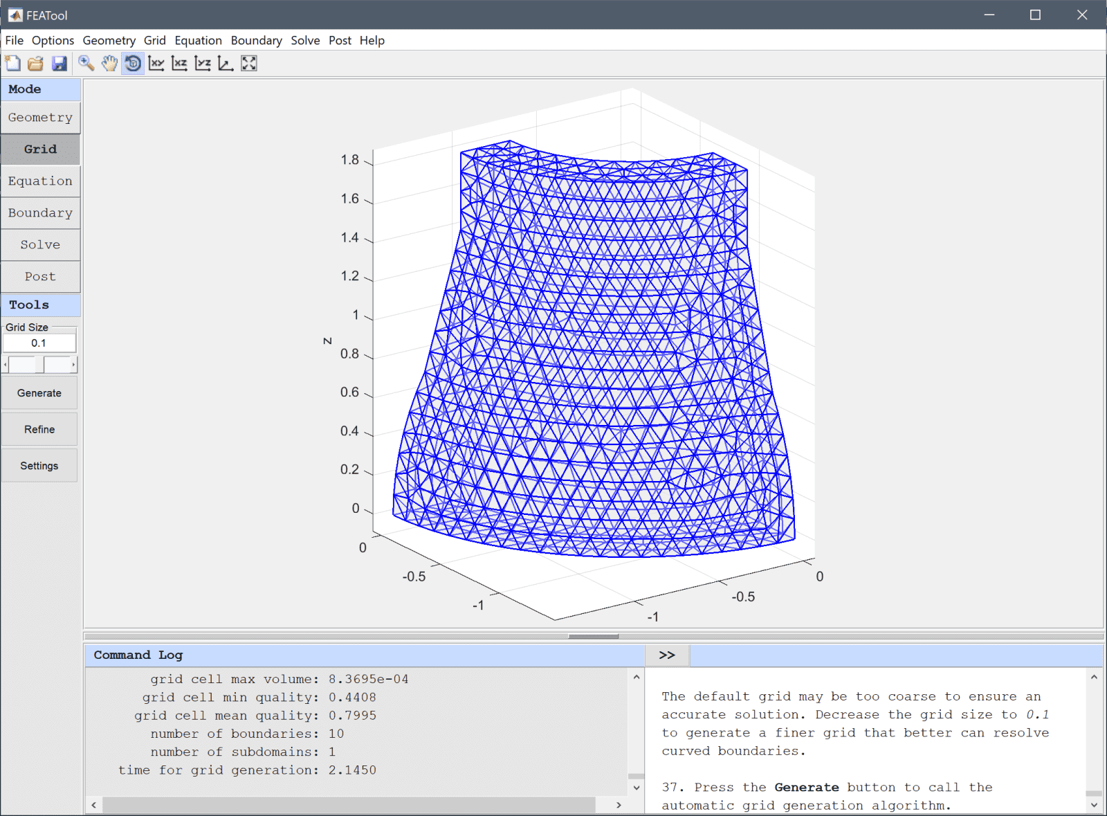
The default grid may be too coarse to ensure an accurate solution. Decrease the grid size to 0.1 to generate a finer grid that better can resolve curved boundaries.

1. Press the Generate button to call the automatic grid generation algorithm.

   
2. Switch to Equation mode by clicking on the corresponding Mode Toolbar button.
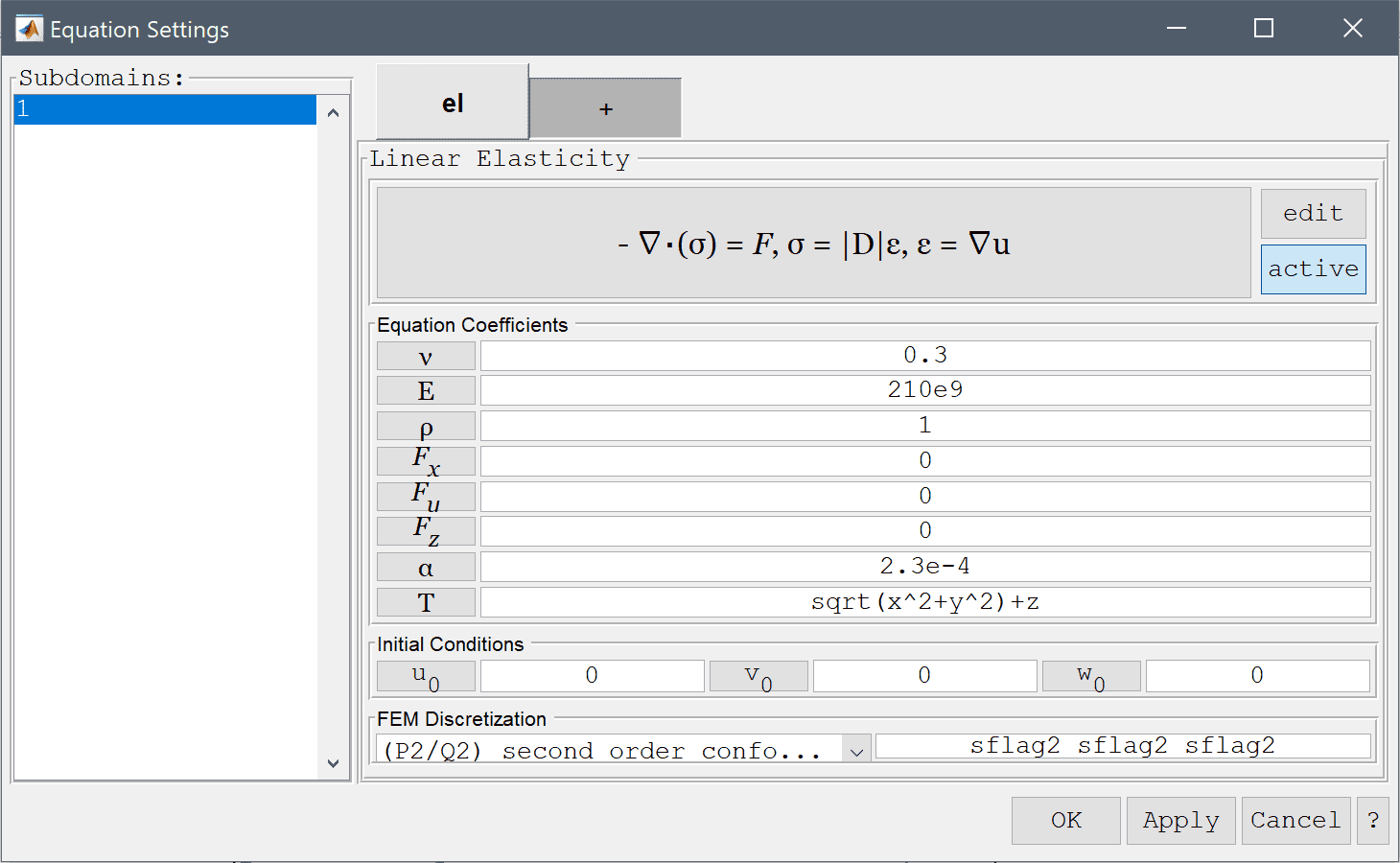
3. Equation and material coefficients can be specified in Equation/Subdomain mode. In the Equation Settings dialog box that automatically opens, enter 0.3 for the Poisson's ratio and 210e9 for the Modulus of elasticity.

Note that FEATool works with any unit system, and it is up to the user to use consistent units for geometry dimensions, material, equation, and boundary coefficients.

The temperature load is a linear expression in the radial direction sqrt(x^2+y^2)+z, but can also be coupled through the temperature from a heat transfer physics mode.

1. Enter 2.3e-4 into the Thermal expansion coefficient edit field.
2. Enter sqrt(x^2+y^2)+z into the Temperature edit field.

As the quantities of interest here are stresses, it is appropriate to use a higher order discretization. This will result in more accurate evaluation of quantities involving derivatives of the solution variables such as stresses.

1. Select (P2/Q2) second order conforming from the FEM Discretization drop-down menu.

   
2. Press OK to finish the equation and subdomain settings specification.
3. Switch to Boundary mode by clicking on the corresponding Mode Toolbar button.

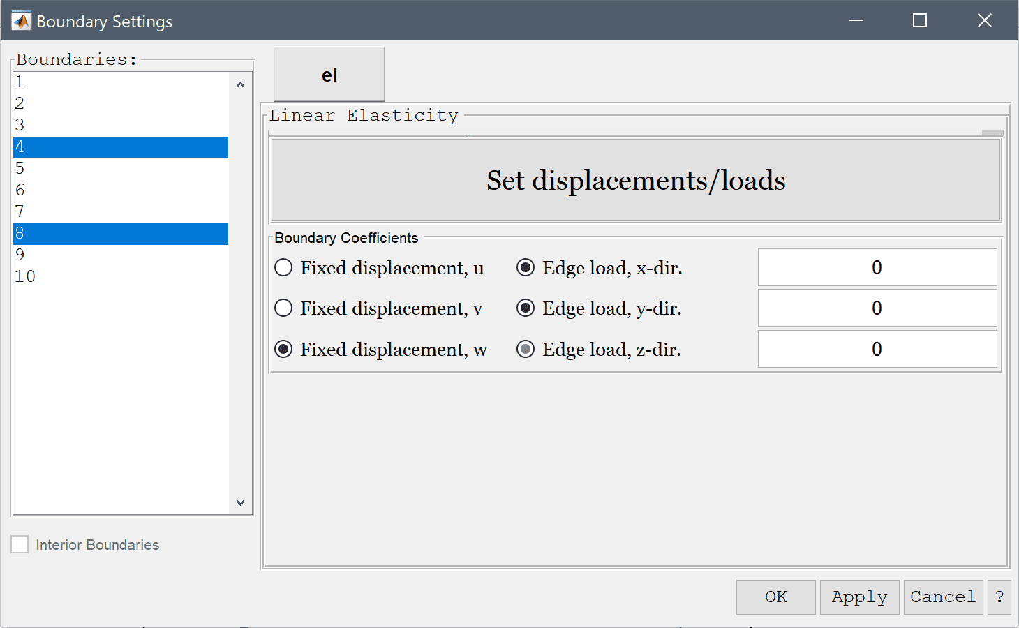
The two side boundaries are due to symmetry, and should therefore have their displacements constrained in the corresponding normal directions.

1. Select 9 in the Boundaries list box.
2. Select the Fixed displacement, v radio button.
3. Select 10 in the Boundaries list box.
4. Select the Fixed displacement, u radio button.

The solid should be clamped in the vertical direction, that is the z-displacement at the top and bottom boundaries should be fixed.

1. Select 4 and 8 in the Boundaries list box.

2. Select the Fixed displacement, w radio button.

   
3. Press OK to finish the boundary condition specification.
4. Switch to Solve mode by clicking on the corresponding Mode Toolbar button.
5. Press the = Toolbar button to call the solver. After the problem has been solved FEATool will automatically switch to postprocessing mode and plot the computed solution.

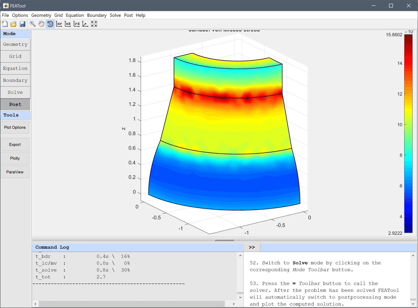
Open the postprocessing settings dialog box and select the z-component of the stress to visualize.

1. Press the Plot Options Toolbar button.
2. Select Stress, z-component from the Predefined surface plot expressions drop-down menu.
3. Press OK to plot and visualize the selected postprocessing options.

4. Press the Go to Y-Z View toolbar button.

   

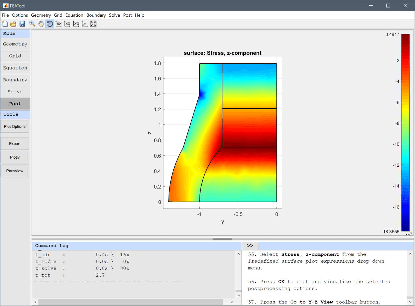
The stress at the inner point (-1, 0, 0) should be evaluated and compared to the reference value.

1. Select Point/Line Evaluation... from the Post menu.
2. Select Stress, z-component from the Evaluation Expression drop-down menu.
3. Enter -1 into the Evaluation coordinates in x-direction edit field.
4. Enter 0 into the Evaluation coordinates in y-direction edit field.

5. Enter 0 into the Evaluation coordinates in z-direction edit field.

   
6. Press OK to finish and close the dialog box.

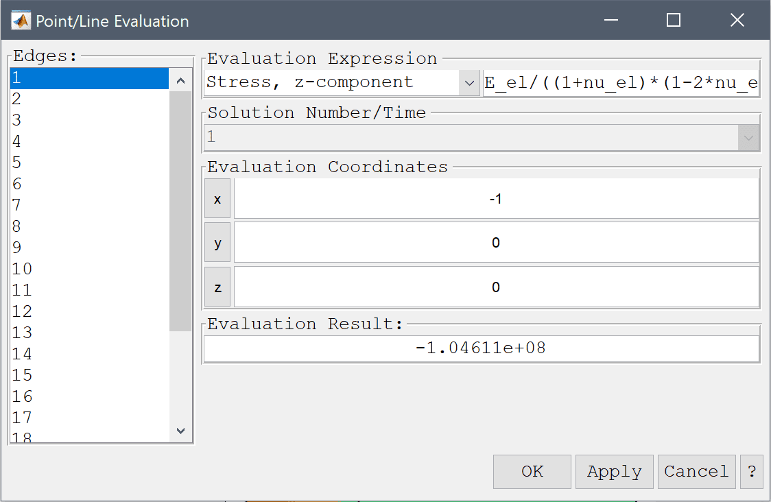
The stress evaluated in the point compares well to the reference value of -105·10⁶ Pa.

The temperature loading of tapered cylinder structural mechanics model has now been completed and can be saved as a binary (.fea) model file, or exported as a programmable MATLAB m-script text file, or GUI script (.fes) file.

Video

Reference

[1] NAFEMS publication TNSB, Rev. 3, The Standard NAFEMS Benchmarks, LE11 Solid Cylinder/Taper/Sphere - Temperature Loading Benchmark, 1990.