To model physical phenomena such as heat transfer, structural stresses, fluid dynamics, chemical reactions, wave propagation and more, a common approach is the continuum model which formulates the problems as partial differential equations. A typical model PDE can be derived by examining the rate of change of the involved quantities in an infinitesimal volume. This chapter introduces some mathematical theory for to derive FEM approach used by FEATool.

Conservation Laws

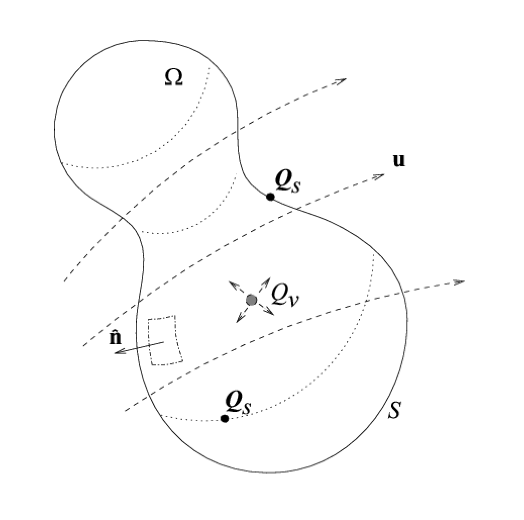
Consider a prototypical property or quantity \(q\), existing in an arbitrary domain \(\Omega\). For this quantity to be conserved within \(\Omega\), the rate of change of \(q\) must be equal to the normal flux crossing the total surface \(S\) (let \(\hat{\mathbf{n}}\) denote the unit normal to \(S\)). With flux meaning the transport of \(q\), in and out of \(\Omega\), with a vector field \(\mathbf{u}\). Any generation from directional surface sources \(\mathbf{Q}_S\) and scalar internal sources \(Q_{V}\) also contributes to an increased (or decreased) amount of \(q\). The following figure illustrates these phenomena for the region \(\Omega\).

A balance equation explicitly stating the conservation of \(q\) will have the form

\[ \frac{\mathrm{net~increase~of~}q}{\mathrm{time}} = \frac{\mathrm{influx}}{\mathrm{time}} + \frac{\mathrm{internal~generation}}{\mathrm{time}} + \frac{\mathrm{surface~generation}}{\mathrm{time}} \]

which is easy to translate into mathematical vector notation

\[ \frac{\partial}{\partial t}\int_{\Omega}q\,d\Omega = -\int_S q\mathbf{u}\cdot\hat{\mathbf{n}}\,dS+\int_{\Omega}Q_{V}\,d\Omega -\int_S \mathbf{Q}_{S}\cdot\hat{\mathbf{n}}\,dS. \]

Application of Gauss' divergence theorem

\[ \int_{S}\mathbf{F}\cdot\hat{\mathbf{n}}\,dS = \int_{\Omega}\nabla\cdot\mathbf{F}\,d\Omega \]

to the surface terms results in the following reformulation

\[ \frac{\partial}{\partial t}\int_{\Omega}q\,d\Omega = -\int_{\Omega}\nabla\cdot q\mathbf{u}\,d\Omega+\int_{\Omega}Q_{V}\,d\Omega -\int_{\Omega}\nabla\cdot\mathbf{Q}_{S}\,d\Omega. \label{eq_cons} \]

Let us consider the conservation of mass by substituting \(q\) with the density \(\rho\). Under the assumption that the system is isolated it is possible to disregard any generation from internal and surface sources. What is left is the following balance equation

\[ \frac{\partial}{\partial t}\int_{\Omega}\rho\,d\Omega = -\int_{\Omega}\nabla\cdot(\rho\mathbf{u})\,d\Omega \]

which must hold for a volume of any size. Thus, in the limit \(\Omega\rightarrow 0\) the well known mass conservation or continuity equation will appear, which reads

\[ \frac{\partial\rho}{\partial t}+\nabla\cdot(\rho\mathbf{u}). \label{eq_ce} \]

Moving on to conservation of linear momentum which, from Newton's second law, is the amount of mass transported with a certain velocity. Specifically, momentum transport per unit volume is therefore expressed as the density \(\rho\) transported with the velocity field \(\mathbf{u}\). If now the product of these quantities is substituted for \(q\) in the general conservation equation then the flux of momentum over the boundaries will accordingly be represented by the quantity \(\rho\mathbf{uu}\). Moreover, momentum is created and destroyed by forces acting internally and on the surface of \(\Omega\). Inside of \(\Omega\) momentum is generated by the presence of forces, here labeled \(\mathbf{f}\), while on the surface momentum is created by both pressure \(p\) and shear stresses, which combined are represented by the stress tensor \(\tau\). Having made these observations enables the following formulation for the conservation of momentum

\[ \frac{\partial}{\partial t} \int_{\Omega}\rho\mathbf{u}\,d\Omega = -\int_{\Omega}\nabla\cdot(\rho\mathbf{uu})\,d\Omega+\int_{\Omega}\mathbf{f}\,d\Omega+ \int_{\Omega}\nabla\cdot\tau\,d\Omega. \]

This should again be valid for a volume of any size or shape with the consequential removal of the integral operations, thus yielding the partial differential equation

\[ \frac{\partial}{\partial t}(\rho\mathbf{u}) = -\nabla\cdot(\rho\mathbf{uu})+\mathbf{f}+\nabla\cdot\tau. \]

The stress tensor \(\tau\) can, as stated above, be subdivided into two parts, the static pressure \(p\) and the shear stresses \(\sigma\). Consider for the moment \(\Omega\) in the form of a unit cube where the coordinate axes are aligned with the surface normals. For a given coordinate axis, the pressure term will now only have one component which is acting directly against the surface normal, while the shear stress terms will have three different components, one in each coordinate direction. This enables a splitting of \(\tau\) into the two terms \(p\mathbf{I}\) and \(\sigma\), that is

\[ \frac{\partial}{\partial t}(\rho\mathbf{u})=-\nabla\cdot(\rho\mathbf{uu})+\mathbf{f}+ \nabla\cdot\left( -p\mathbf{I}+ \sigma \right) \label{eq_linmom} \]

where \(\mathbf{I}\) denotes the diagonal unit matrix.

Poisson Equation

The Poisson equation is a very good model equation to study since it can represent many different physical processes such as diffusion, thermal conduction, and electric potential. The following example illustrates how to set up and solve the Poisson equation on a unit sphere \(-D\Delta u=1\) ( \(r=0..1\)) with homogeneous boundary conditions, that is \(u=0|_{r=1}\).

To derive the finite element discretization of the general Poisson equation \(-\Delta u = f\) first multiply the equation with an arbitrary function \(v\) (called test function), and integrate over the whole domain \(\Omega\), that is \(\int_{\Omega} -\Delta u v\ d\Omega=\int_{\Omega} fv\ d\Omega\). By applying the Gauss theorem or partial integration to the left side we get

\[ \int_{\Omega} \nabla u\cdot\nabla v\ d\Omega + \int_{\partial\Omega} -\hat{\textbf{n}}\cdot\nabla u\ dS=\int_{\Omega} fv\ d\Omega \]

The boundary term can be neglected assuming that we only have prescribed or fixed value (Dirichlet) boundary conditions. In 2D the equation will look like

\[ \int_{\Omega} \frac{\partial u}{\partial x}\frac{\partial v}{\partial x}+\frac{\partial u}{\partial y}\frac{\partial v}{\partial y}\ dxdy = \int_{\Omega} fv\ dxdy \]

By discretizing the solution (trial function space) variable as \(u=\sum_{i=1}^N \phi_i u_i\) and similarly test function \(v=\sum_{j=1}^N \phi_j\), where \(\phi_{i/j}\) are the finite element shape or basis functions (usually taken the same for \(i\) and \(j\) in the Galerkin approximation), and \(u_i\) is the value of the solution at node \(i\). Inserting this we get

\[ \int\sum_{i=1}^N\sum_{j=1}^N \frac{\partial \phi_i}{\partial x}\frac{\partial \phi_j}{\partial x}+\frac{\partial \phi_i}{\partial y}\frac{\partial \phi_j}{\partial y}\ u_i = \int\sum_{j=1}^N f\phi_j \]

which after discretization and integration with numerical quadrature gives us a matrix system to solve

\[ Au=b \]

Boundary and Initial Conditions

The modeled applications and processes are usually very specific in nature and the studies can thus be confined to a smaller spatial sub region or domain \(\Omega \subset \mathbf{R}^d\) and a specific temporal extent \([0,T]\). Both these restrictions will usually greatly simplify the modeling and also reduce the effort required to obtain a solution. It is particularly advantageous to utilize all existing symmetry axes to further shrink the computational domain. Sometimes it is also possible to transform a three dimensional model to two dimensions if the problem can be considered axisymmetric. The drawback of restricting the models spatially is that the equations now have to be supplied with suitable boundary conditions, which goal is to describe all interactions between \(\Omega\) and the rest of the non-modeled environment.

Boundary conditions usually come in two distinct variants, Dirichlet conditions which fixes the value of a quantity

\[ u = r \quad on \quad \partial\Omega_D. \]

and Neumann, also called natural, boundary conditions which specify the in- or outward-flux

\[ \hat{-\mathbf{n}}\cdot D\nabla u = g \quad on \quad \partial\Omega_N. \]

Initial conditions, in the form of specified \(u(\mathbf{x},0) = u_0(\mathbf{x})\), must be prescribed in addition to the boundary conditions for applications where the temporal evolution is of interest. For non-linear stationary calculations it is also advantageous to specify a good initial guess so that the nonlinear solver will converge faster.

Internal Boundary Conditions

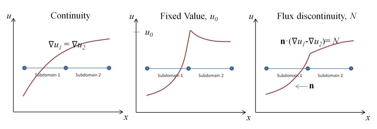
A note on boundary conditions on internal boundaries, that is boundaries shared between two subdomnains. (Check the Interior Boundaries checkbox in the Boundary Settings dialog box to activate selection on internal boundaries.) There are in general three types of boundary conditions available to set on these boundaries

Continuity, meaning that the difference in flux or gradient between two boundaries is zero (homogeneous Neumann). This is the default and usual condition for all boundaries unless one of the other conditions are prescribed.
Fixed value, is a Dirichlet condition prescribing specific value on the internal boundaries.
Flux discontinuity, prescribes the difference in the flux/gradient between the two sides. This condition would only be used in rare instance where one for some reason must prescribe a difference in the gradient.

See the image below for an explanation of the boundary conditions available to set on internal boundaries (the normal on internal boundaries is defined as pointing from the subdomain with higher number to lower). Note that is is not possible to directly prescribe and set the gradient/flux on internal boundaries (as it is for external ones).

Poisson Example

A tutorial example for the Poisson equation on a unit line can be found in the Poisson Equation tutorial section. This example is split up into four parts showing how set up and solve the model in the GUI, as well as on the command line using physics modes, and the CLI Tutorial Using Core FEM Library Functions highlighting use of FEM library functions such as matrix assembly.