The classic Poisson equation is one of the most fundamental partial differential equations (PDEs). Although one of the simplest equations, it is a very good model for the process of diffusion and comes up in many applications (for example fluid flow, heat transfer, and chemical transport). It is therefore fundamental to many simulation codes to be able to solve it efficiently and accurately.

This example shows how to set up and solve the Poisson equation

\[ d_{ts}\frac{\partial u}{\partial t} + \nabla\cdot(-D\nabla u) = f \]

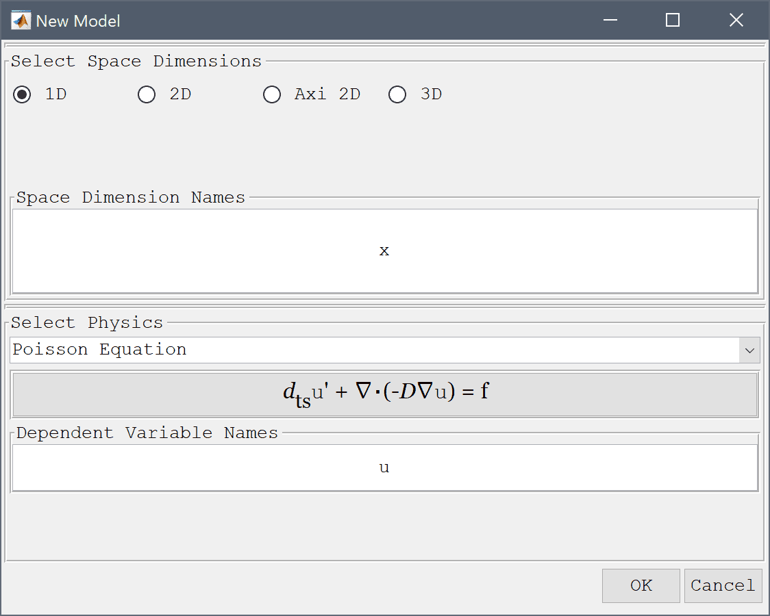
for a scalar field u = u(x) on a unit line. Both the diffusion coefficient D and right hand side source term f are assumed to be constant and equal to 1. The Poisson problem is also considered stationary meaning that the time dependent term can be neglected. Homogeneous Dirichlet boundary conditions, u = 0 are prescribed on all boundaries of the domain. The exact solution for this problem is u(x) = (-x²+x)/2 which can be used to measure the accuracy of the computed solution.

Tutorial

This model is available as an automated tutorial by selecting Model Examples and Tutorials... > Classic PDE > Poisson Equation from the File menu. Or alternatively, follow the video tutorial or step-by-step instructions below.

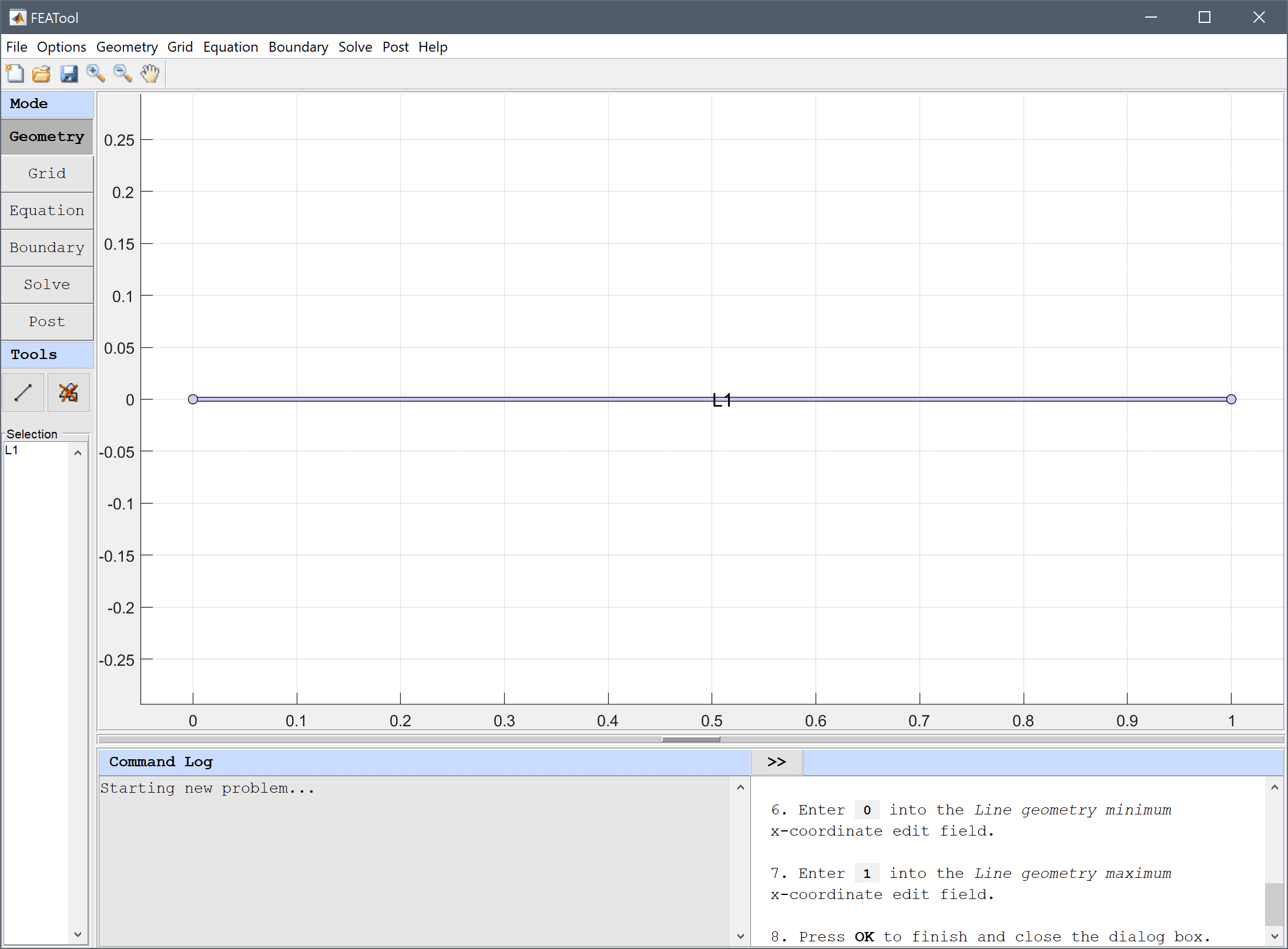
To start a new model click the New Model toolbar button, or select New Model... from the File menu.
Select the 1D radio button.
Select the Poisson Equation physics mode from the Select Physics drop-down menu.
Press OK to finish the physics mode selection.
Press the Create line Toolbar button.
Enter 0 into the Line geometry minimum x-coordinate edit field.
Enter 1 into the Line geometry maximum x-coordinate edit field.
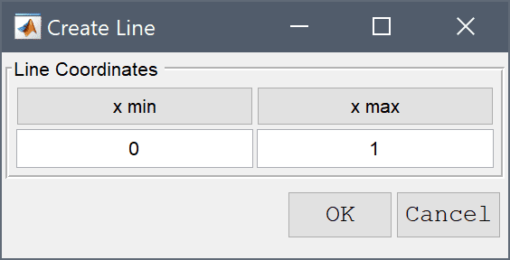
Press OK to finish and close the dialog box.
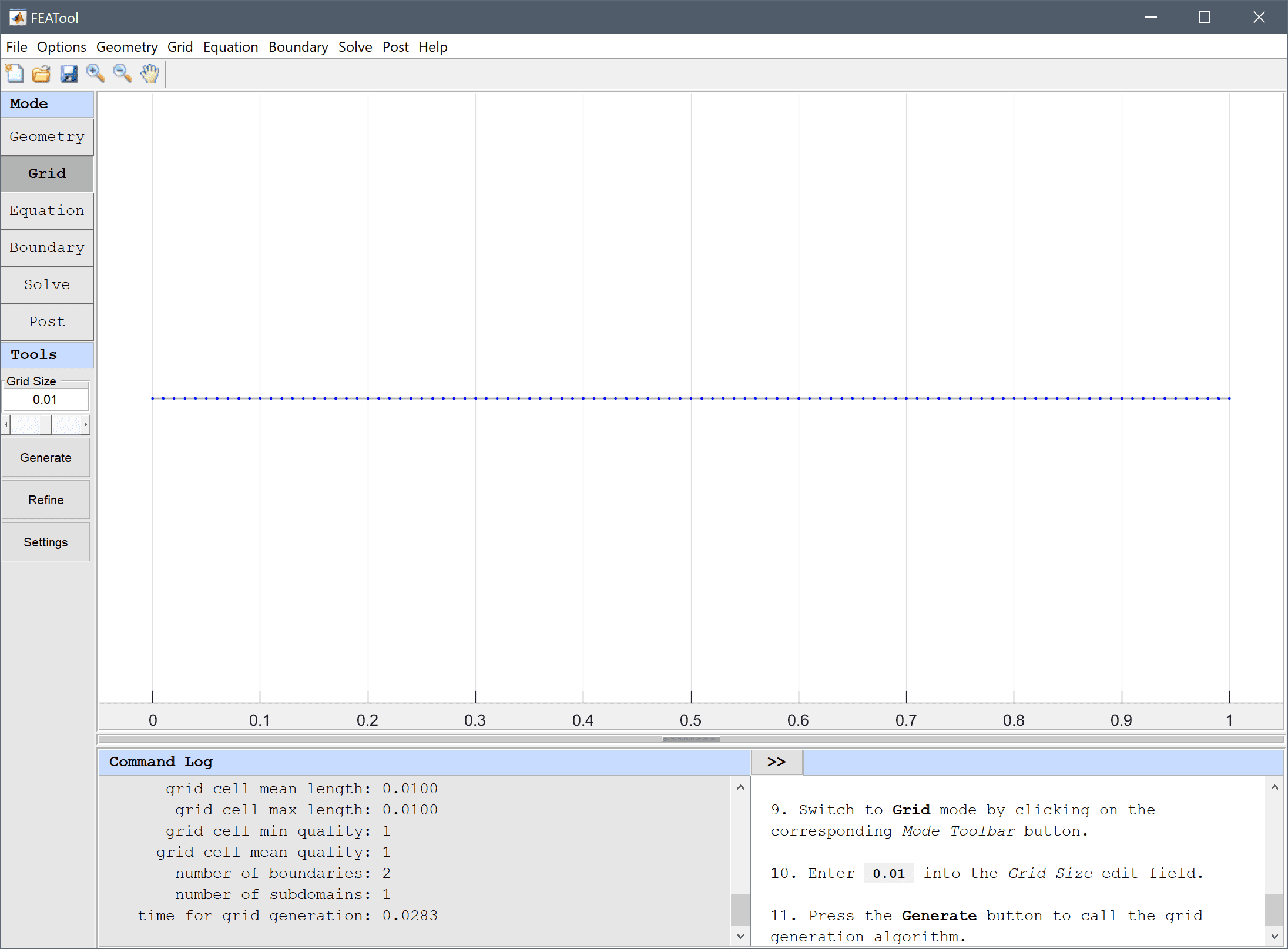
Switch to Grid mode by clicking on the corresponding Mode Toolbar button.
Enter 0.01 into the Grid Size edit field and press the Generate button to call the grid generation algorithm.
Switch to Equation mode by clicking on the corresponding Mode Toolbar button.
Enter 1 into the Diffusion coefficient edit field, and 1 into the Source term edit field.
Press OK to finish the equation and subdomain settings specification.
Switch to Boundary mode by clicking on the corresponding Mode Toolbar button.
Select 1 and 2 in the Boundaries list box.
Select Dirichlet boundary condition from the Poisson Equation drop-down menu.
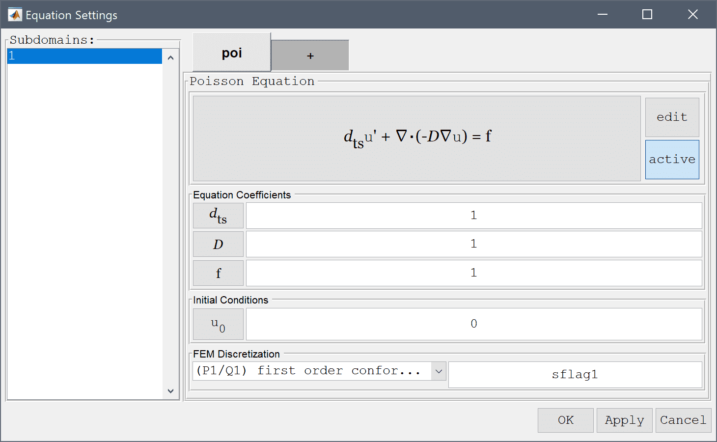
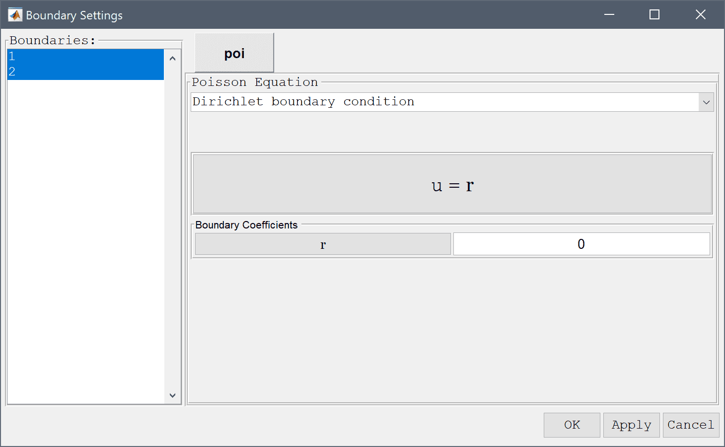
Enter 0 into the Dirichlet coefficient edit field.
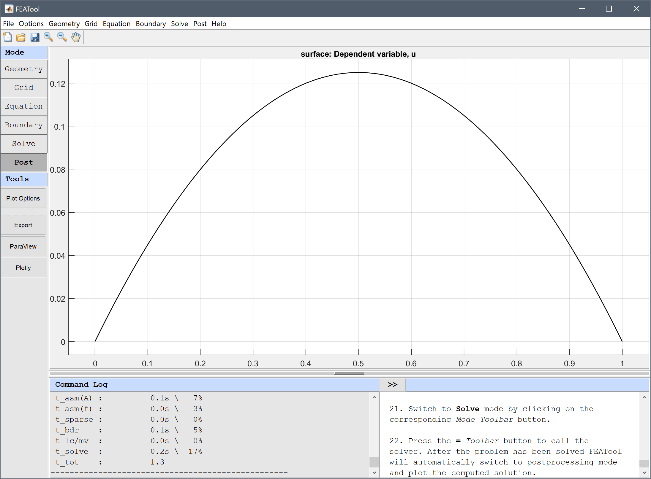
Press OK to finish the boundary condition specification.
Switch to Solve mode by clicking on the corresponding Mode Toolbar button.
Press the = Toolbar button to call the solver. After the problem has been solved FEATool will automatically switch to postprocessing mode and plot the computed solution.

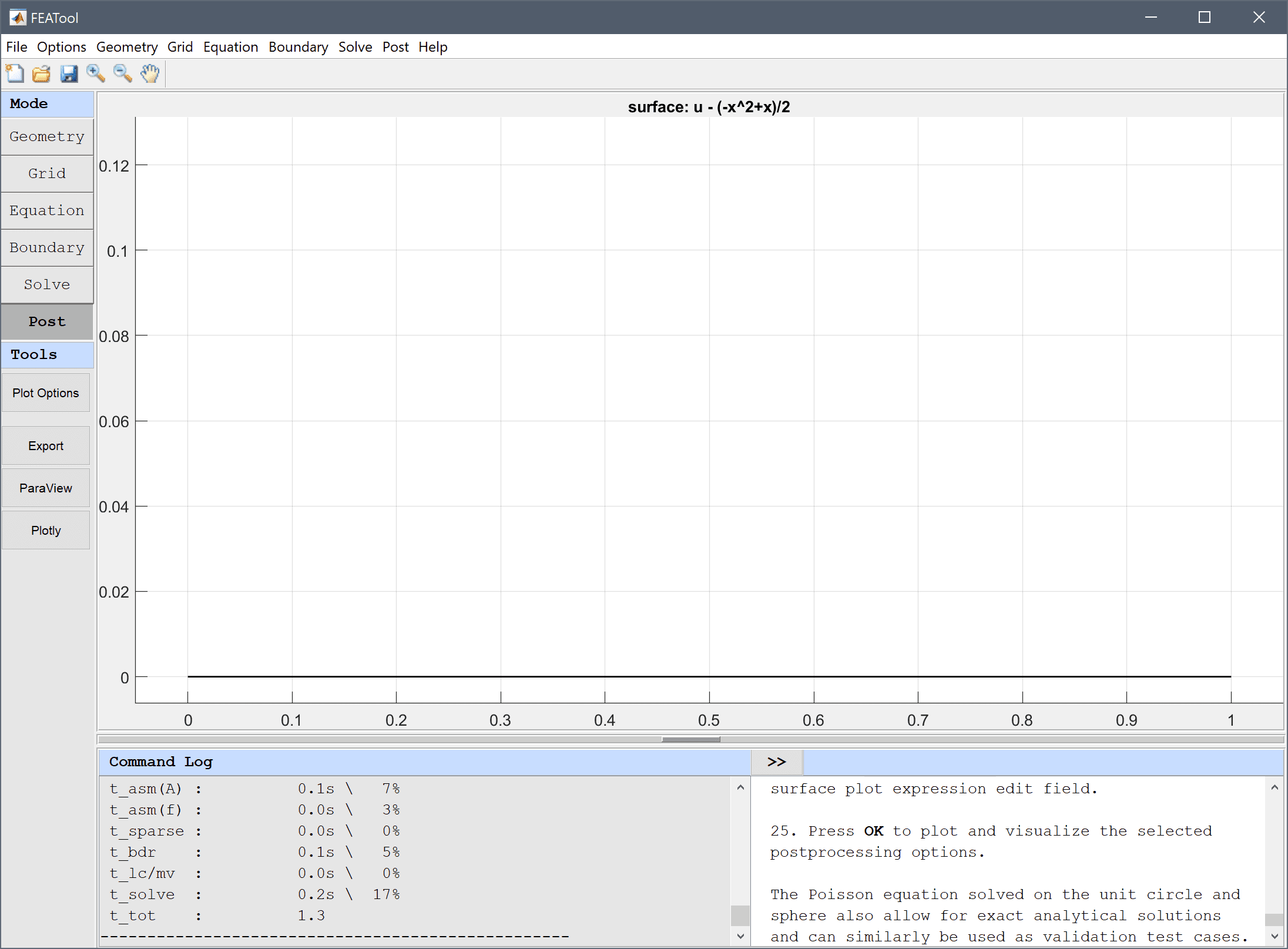
To visualize the error, plot the difference between the computed solution and the exact analytical solution u - (-x²+x)/2.

Press the Plot Options Toolbar button.
Enter u - (-x^2+x)/2 into the User defined surface plot expression edit field.
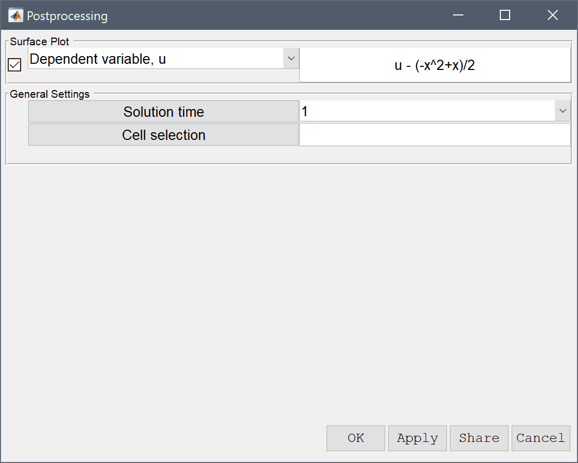
Press OK to plot and visualize the error.

Similar to this example, the Poisson equation solved for the unit circle and sphere also allow for exact analytical solutions, and can similarly be used as PDE validation test cases.

The Poisson equation solved on the unit circle and sphere also allow for exact analytical solutions and can similarly be used as validation test cases.

The classic poisson equation PDE model has now been completed and can be saved as a binary (.fea) model file, or exported as a programmable MATLAB m-script text file (available as the example ex_poisson1 script file), or GUI script (.fes) file.

Video

CLI Tutorial Using Physics Modes

This section describes how to set up and solve the Poisson equation with the MATLAB command line interface (CLI). To make it easier and faster for users to set up model problems several physics modes have been predefined with equations and boundary conditions for physics such as convection, diffusion, and reaction of chemical species, heat transport through convection and conduction, and incompressible fluid flow with the Navier-Stokes equations. In this example the Poisson physics mode will be used.

Start MATLAB and make sure you have either run the installation script to set up the FEATool directory paths or alternatively run
```
addpaths
```
on the command line from the FEATool installation directory before you start.

Define a unit line geometry object

 gobj = gobj_line( [0; 1] );
 fea.geom.objects  = { gobj };

Call gridgen to create an unstructured grid with maximum grid cell size hmax

 hmax     = 0.01;   % Maximum grid cell size.
 fea.grid = gridgen( fea, 'hmax', hmax );

Assign a name to the space dimension coordinate (these names can then be used in equation coefficients and postprocessing expressions)
```
 fea.sdim = { 'x' };
```
Use addphys to add the predefined Poisson physics mode
```
 fea = addphys( fea, @poisson );
```
To find and set the diffusion coefficient and source term to 1 first Inspect the eqn.coef field and verify that the d_poi coefficient and f_poi source term are assigned rows 2 and 3, respectively. The coefficients values are specified in the fourth column of eqn.coef as a cell array of values per subdomain (in this case only one subdomain)
```
 fea.phys.poi.eqn.coef
```

Now set the equation coefficients

 fea.phys.poi.eqn.coef{2,4} = {1};   % Diffusion coefficient.
 fea.phys.poi.eqn.coef{3,4} = {1};   % Source term.

To find and set the Dirichlet boundary coefficients to 0, first inspect the bdr.coef field and verify that the Dirichlet conditions are used with the coefficient set to zero
```
 fea.phys.poi.bdr.coef
```

Then set the correct boundary coefficients

 % Use first boundary condition specification
 % (Dirchlet) for both boundary end points.
 fea.phys.poi.bdr.sel = [ 1, 1 ];

 % Set the Dirichlet coefficients to zero.
 fea.phys.poi.bdr.coef{1,end} = { 0, 0 };

Check and parse the physics and problem structs by calling parsephys and parseprob (this verifies that everything in the problem definition struct is correct and outputs the necessary lower hierarchy fields)
```
fea = parsephys( fea );
fea = parseprob( fea );
```
Call the stationary solver solvestat with the default settings
```
fea.sol.u = solvestat(fea);
```
Plot with postplot to display and visualize the scalar solution as a surface plot
```
postplot( fea, 'surfexpr', 'u' )
```

Plot the difference between the computed and exact solution

u_diff = 'u - (-x^2+x)/2';
clf
postplot( fea, 'surfexpr', u_diff )

CLI Tutorial Without Physics Modes

This section describes how to set up and solve the Poisson equation with the MATLAB command line interface (CLI) by directly setting up the necessary equation and boundary definition fields (that is without using the predefined Poisson physics mode).

Start MATLAB and make sure you have either run the installation script to set up the FEATool directory paths or alternatively run
```
 addpaths
```
on the command line from the FEATool installation directory before you start.

Define a unit line geometry object

 gobj = gobj_line( [0; 1] );
 fea.geom.objects  = { gobj };

Call gridgen to create an unstructured grid with maximum grid cell size hmax

 hmax     = 0.01;   % Maximum grid cell size.
 fea.grid = gridgen( fea, 'hmax', hmax );

Assign a name to the space dimension coordinate (these names can then be used in equation coefficients and postprocessing expressions)
```
 fea.sdim = { 'x' };
```
Assign a name to the dependent variable (in this case u)
```
 fea.dvar = { 'u' };
```
Define a finite element shape function to use for the discretization (here sflag1 corresponds to linear conforming P1 finite element shape functions, while sflag2 would correspond to second order P2 shape functions.)
```
 fea.sfun = { 'sflag1' };
```

Define the equation system, bilinear form in fea.eqn.a and right hand side linear form in fea.eqn.f

 % Define bilinear form. The first row indicates test function
 % space, and second row trial function space. Each column
 % defines a term in the bilinear form and 1 corresponds to
 % a basis function evaluation, 2 = x-derivative,
 % (3 = y-derivative in 2D, and 4 = z-derivative in 3D).
 fea.eqn.a.form = { [2; 2] };

 % Define coefficients used in assembling the bilinear forms.
 fea.eqn.a.coef = { [1 1] };

 % Test function space to evaluate in linear form.
 fea.eqn.f.form = { 1 };

 % Coefficient value used in assembling the linear form.
 fea.eqn.f.coef = { 1 };

Define the boundary conditions, Dirichlet conditions in fea.bdr.d and Neumann (flux conditions) in fea.bdr.n

 % Number of boundary segments.
 n_bdr = max(fea.grid.b(3,:));

 % Allocate space for n_bdr boundaries.
 fea.bdr.d = cell(1,n_bdr);

 % Assign u=0 to all Dirichlet boundaries.
 [fea.bdr.d{:}] = deal(0);

 % No Neumann boundaries (fea.bdr.n{i} empty).
 fea.bdr.n      = cell(1,n_bdr);

Check and parse the problem struct by calling parseprob (this verifies that everything in the problem definition struct is correct and outputs the necessary lower hierarchy fields)
```
 fea = parseprob( fea );
```
Call the stationary solver solvestat with the default settings
```
fea.sol.u = solvestat( fea );
```
Plot with postplot to display and visualize the scalar solution as a surface plot
```
postplot( fea, 'surfexpr', 'u' )
```

Plot the difference between the computed and exact solution

u_diff = 'u - (-x^2+x)/2';
clf
postplot( fea, 'surfexpr', u_diff )

CLI Tutorial Using Core FEM Library Functions

This final section shows how to define and solve the Poisson equation by directly calling the core finite element library functions. The low level functions are used to assemble the system matrix and right hand side vector to which boundary conditions are applied, after which the system can be solved.

Start MATLAB and make sure you have either run the installation script to set up the FEATool directory paths or alternatively run
```
 addpaths
```
on the command line from the FEATool installation directory before you start.

Define a unit line geometry object

 gobj = gobj_line( [0; 1] );
 fea.geom.objects  = { gobj };

Call gridgen to create an unstructured grid with maximum grid cell size hmax

 hmax     = 0.01;   % Maximum grid cell size.
 fea.grid = gridgen( fea, 'hmax', hmax );

Use the function assemblea to assemble the finite element stiffness matrix

 % Bilinear form to assemble (u_x*v_x).
 form  = [2;2];

 % FEM shape functions used in test and trial function spaces
 % (here first order conforming P1 Lagrange functions).
 sfun  = {'sflag1';'sflag1'};

 % Coefficients to use for each term in the bilinear form.
 coef  = [1 1];
 i_cub = 3;   % Numerical quadrature rule to use.

 [vRowInds,vColInds,vAvals,n_rows,n_cols] = ...
      assemblea( form, sfun, coef, i_cub,  ...
        fea.grid.p, fea.grid.c, fea.grid.a );

 % Construct sparse matrix.
 A = sparse( vRowInds, vColInds, vAvals, n_rows, n_cols );

Assemble right hand side load vector by calling assemblef

 % Linear form to assemble (1 = evaluate function values).
 form  = [1];

 % Finite element shape function.
 sfun  = {'sflag1'};

 % Coefficient to use in the linear form.
 coef  = [1];

 % Numerical quadrature rule to use.
 i_cub = 3;

 f = assemblef( form, sfun, coef, i_cub, ...
       fea.grid.p, fea.grid.c, fea.grid.a );

Find indexes to boundary nodes

 bind = [];
 for i_b=1:size(fea.grid.b,2)    % Loop over boundary edges.
   i_c    = fea.grid.b(1,i_b);   % Cell number.
   i_edge = fea.grid.b(2,i_b);
   j_edge = mod( i_edge, size(fea.grid.c,1) ) + 1;
   bind   = [bind fea.grid.c([i_edge j_edge],i_c)'];
 end
 bind = unique(bind);

Set homogeneous Dirichlet boundary conditions

 A = A';   % Transpose matrix for faster row elimination.
 A(:,bind) = 0;          % Zero/remove entire rows.
 for i=1:length(bind)    % Set diagonal entries of Dirichlet
                         % boundary condition rows to 1.
   i_a        = bind(i);
   A(i_a,i_a) = 1;
 end
 A = A';

 f(bind) = 0;            % Set corresponding RHS entries
                         % to the prescribed boundary values.

Solve (invert) problem by calling the built-in linear solver
```
 u = A\f;
```

Create fea help fields for postprocessing

 fea.sdim  = { 'x' };
 fea.dvar  = { 'u' };
 fea.sfun  = { 'sflag1' };
 fea       = parseprob( fea );

Use postplot to plot the solution

fea.sol.u = u;
postplot( fea, 'surfexpr', 'u' )

Plot the difference between the computed and exact solution

x = fea.grid.p(1,:);
u_diff = u - (-x.^2+x)/2;
clf
fea.sol.u = u_diff;
postplot( fea, 'surfexpr', 'u' )

Poisson Equation for a Circle with a Point Source

The Poisson Equation with a Point Source example shows how to model a Poisson equation on a circle with a point source at its center.

Poisson Equation for a Sphere

The following example illustrates how to set up and solve the Poisson equation on a unit sphere \(-\Delta u=1\) ( \(r=0..1\)) with homogeneous boundary conditions, that is \(u=0|_{r=1}\) with the FEATool FEM assembly primitives.

To derive the finite element discretization of the general Poisson equation \( -\Delta u = f\) first multiply the equation with an arbitrary function \(v\) (called test function), and integrate over the whole domain \(\Omega\), that is \(\int_{\Omega} -\Delta u v\ d\Omega=\int_{\Omega} fv\ d\Omega\). By applying the Gauss theorem or partial integration to the left side we get

\[ \int_{\Omega} \nabla u\cdot\nabla v\ d\Omega + \int_{\partial\Omega} -\hat{\bf{n}}\cdot\nabla u\ dS=\int_{\Omega} fv\ d\Omega \]

The boundary term can be neglected assuming that we only have prescribed or fixed value (Dirichlet) boundary conditions. In 3D the equation will look like

\[ \int_{\Omega} \frac{\partial u}{\partial x}\frac{\partial v}{\partial x}+\frac{\partial u}{\partial y}\frac{\partial v}{\partial y}+\frac{\partial u}{\partial z}\frac{\partial v}{\partial z}\ dxdydz = \int_{\Omega} fv\ dxdydz \]

By discretizing the solution (trial function space) variable as \(u=\sum_{i=1}^N \phi_i u_i\) and similarly test function \(v=\sum_{j=1}^N \phi_j\), where \(\phi_{i/j}\) are the finite element shape or basis functions (usually taken the same for \(i\) and \(j\) in the Galerkin approximation), and \(u_i\) is the value of the solution at node \(i\). Inserting this we get

\[ \int\sum_{i=1}^N\sum_{j=1}^N \frac{\partial \phi_i}{\partial x}\frac{\partial \phi_j}{\partial x}+\frac{\partial \phi_i}{\partial y}\frac{\partial \phi_j}{\partial y}+\frac{\partial \phi_i}{\partial z}\frac{\partial \phi_j}{\partial z}\ u_i = \int\sum_{j=1}^N f\phi_j \]

which after discretization and integration with numerical quadrature gives us a matrix system to solve

\[ Au=b \]

To start implementing the model pragmatically we first have to create a grid. Instead of creating a grid by using a geometry object we use a geometric sphere grid primitive directly

grid = spheregrid();
p = grid.p;   % Extract grid points.
c = grid.c;   % Extract grid cells.
a = grid.a;   % Extract adjacency information.

To assemble the matrix A we can identify three bi-linear terms (with a coefficient of one) \(1\cdot\phi_{i,x}\phi_{i,y}+1\cdot\phi_{i,y}\phi_{j,y}+1\cdot\phi_{i,z}\phi_{j,z}\). To specify this in FEATool first create a cell array with coefficient values (or expressions) for each term, in this case coef = {1 1 1};. Function values and/or derivatives for the trial and test functions are specified in a 2 by n-terms vector, here form = [2 3 4;2 3 4]; where the first row specifies trial functions to use for the three terms (1=function value, 2=x-derivative, 3=y-derivative, 4=z-derivative), and the bottom row the test functions. Lastly, the actual shape or basis functions are specified in a cell array as sfun = {'sflag1';'sflag1'};, which prescribes first order linear Lagrange shape functions for both the trial and test function spaces. Given a grid with grid points p and cell connectivity c the call to the fem assembly routine looks like

coef   = { 1 1 1 };
form   = [ 2 3 4 ; ...
           2 3 4 ];
sfun   = { 'sflag1' ; ...
           'sflag1' };
i_cub  = 3;              % Numerical quadrature rule.
cind   = 1:size(c,2);    % Index to cells to assemble.
[i,j,s,m,n] = assemblea( form, sfun, coef, i_cub, p, c, a );
A      = sparse( i, j, s, m, n );

Similarly, the right hand side linear form or load vector b can be assembled as

coef   = { 1 };
form   = [ 1 ];
sfun   = { 'sflag1' };
i_cub  = 3;              % Numerical quadrature rule.
cind   = 1:size(c,2);    % Index to cells to assemble.
b      = assemblef( form, sfun, coef, i_cub, p, c, a );

Prescribing homogeneous (zero value) Dirichlet boundary conditions on the boundary of the domain can be done by first finding the indexes to the nodes on the boundary (in this case the unit sphere), and then setting the corresponding values in the load vector to zero. Moreover, the corresponding rows in the matrix A must also be modified so that they are all zero except for the diagonal entries which are set to one (this preserves the boundary values specified in the b vector).

radi = sqrt(sum(p.^2,1));        % Radius of grid points.
bind = find(radi>1-sqrt(eps));   % Find grid points
                                 % on the boundary.

b(bind)   = 0;            % Set 'bind' rhs entries to zero.

A(bind,:) = 0;            % Set 'bind' rows to zero.
for i=1:length(bind)      % Set 'bind' diagonal entries to 1
  i_a        = bind(i);
  A(i_a,i_a) = 1;
end

The problem is now fully specified and can be solved as

u = A\b;

where u now contains the values of the solution in the grid points/nodes. To visualize the solution we put everything in a FEATool fea struct

fea.grid  = grid;
fea.dvar  = { 'u' };
fea.sfun  = sfun;
fea.sol.u = u;
fea = parseprob( fea );

postplot( fea, 'surfexpr', 'u', 'selcells', 'y>-0.1' )