|
FEATool Multiphysics
v1.16.5
Finite Element Analysis Toolbox
|
|
FEATool Multiphysics
v1.16.5
Finite Element Analysis Toolbox
|
This is an example showing how to define a custom PDE equation model in the FEATool Multiphysics. In this case the Black-Scholes model equation, which is used in financial analytics to model derivatives and options pricing. The non-linear partial differential equation to be solved reads
\[ \frac{\partial u}{\partial t} - \frac{\partial}{\partial x}(\frac{1}{2}\frac{\partial u}{\partial x}) - \frac{\partial u}{\partial x} = -u + ( (x-t)^5 - 10(x-t)^4 - 10(x-t)^3) \]
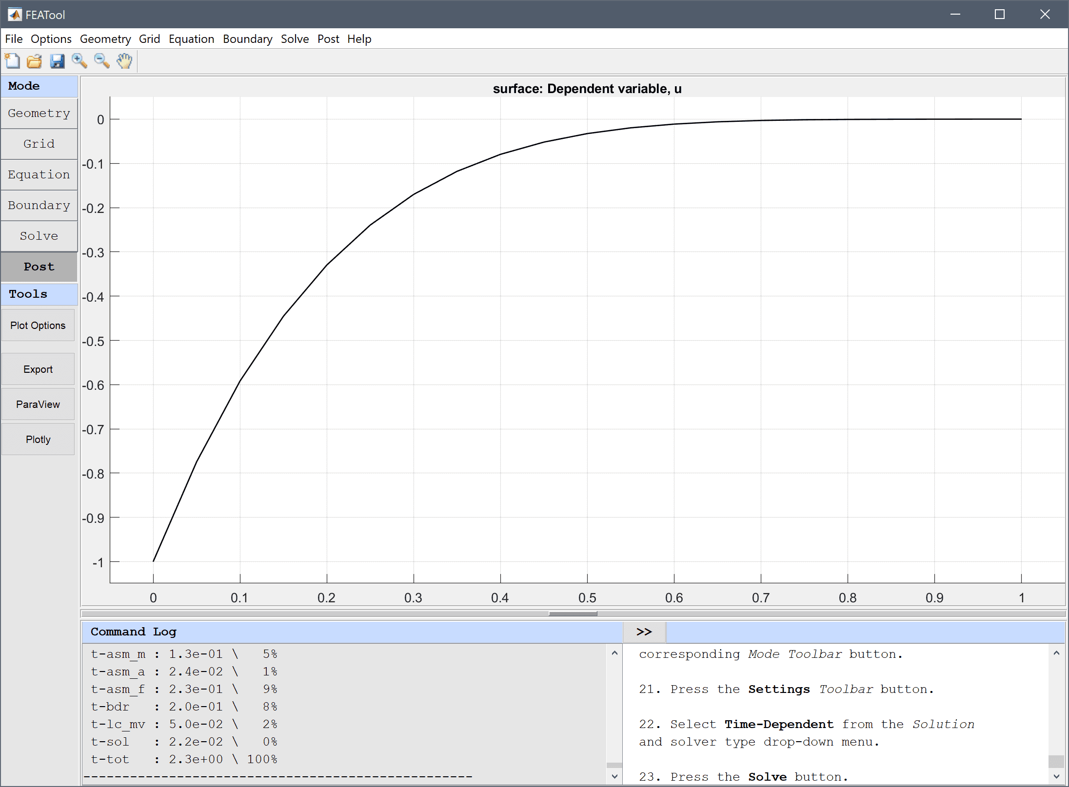
with boundary conditions u(0,t) = -t^5 and u(x,t) = (x-t)^5 on the left and right sides of the domain, respectively. The problem is time-dependent with initial condition is u(x,t=0) = x^5. For this problem an exact analytical solution exists, u(x,t) = (x-t)^5, which can be used to verify the computed solution. See the Custom Equation section for details on the equation syntax.
This model is available as an automated tutorial by selecting Model Examples and Tutorials... > Classic PDE > Black-Scholes Equation from the File menu, viewed as a videotutorial", or alternatively, follow the step-by-step instructions below.
Select the Custom Equation physics mode from the Select Physics drop-down menu.
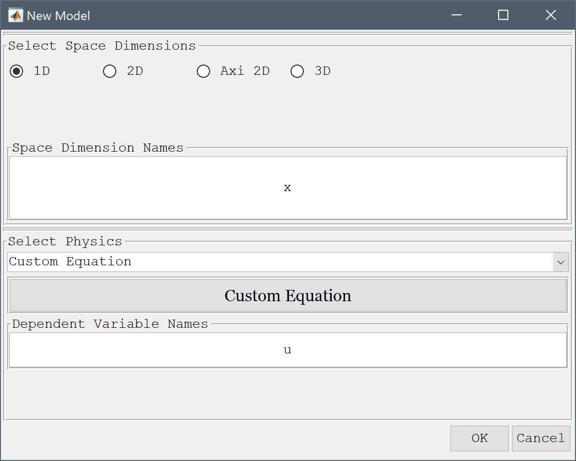
Press OK to finish and close the dialog box.

Press the Generate button to call the grid generation algorithm.

Enter u' - 1/2*ux_x - ux_t + u_t = (x-t)^5 - 10*(x-t)^4 - 10*(x-t)^3 into the Equation for u edit field.

Enter x^5 into the Initial condition for u edit field.

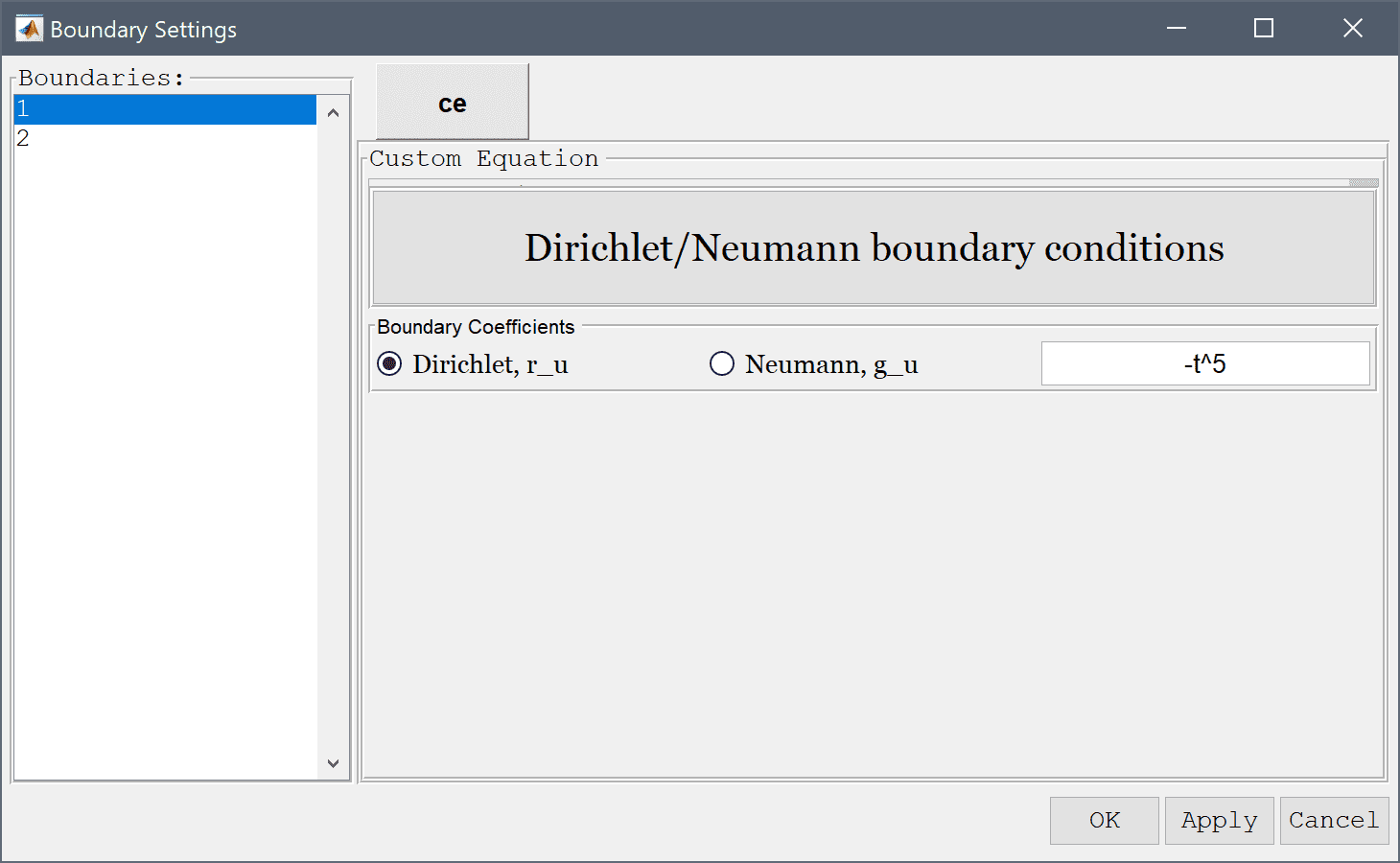
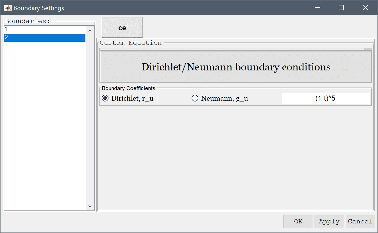
The values at the two boundaries should be set to -t^5 minus t to the power of 5, at the left boundary, and (1-t)^5 to the right, where t represents time.
Enter -t^5 into the Dirichlet/Neumann coefficient edit field.
Enter (1-t)^5 into the Dirichlet/Neumann coefficient edit field.
Select Time-Dependent from the Solution and solver type drop-down menu.
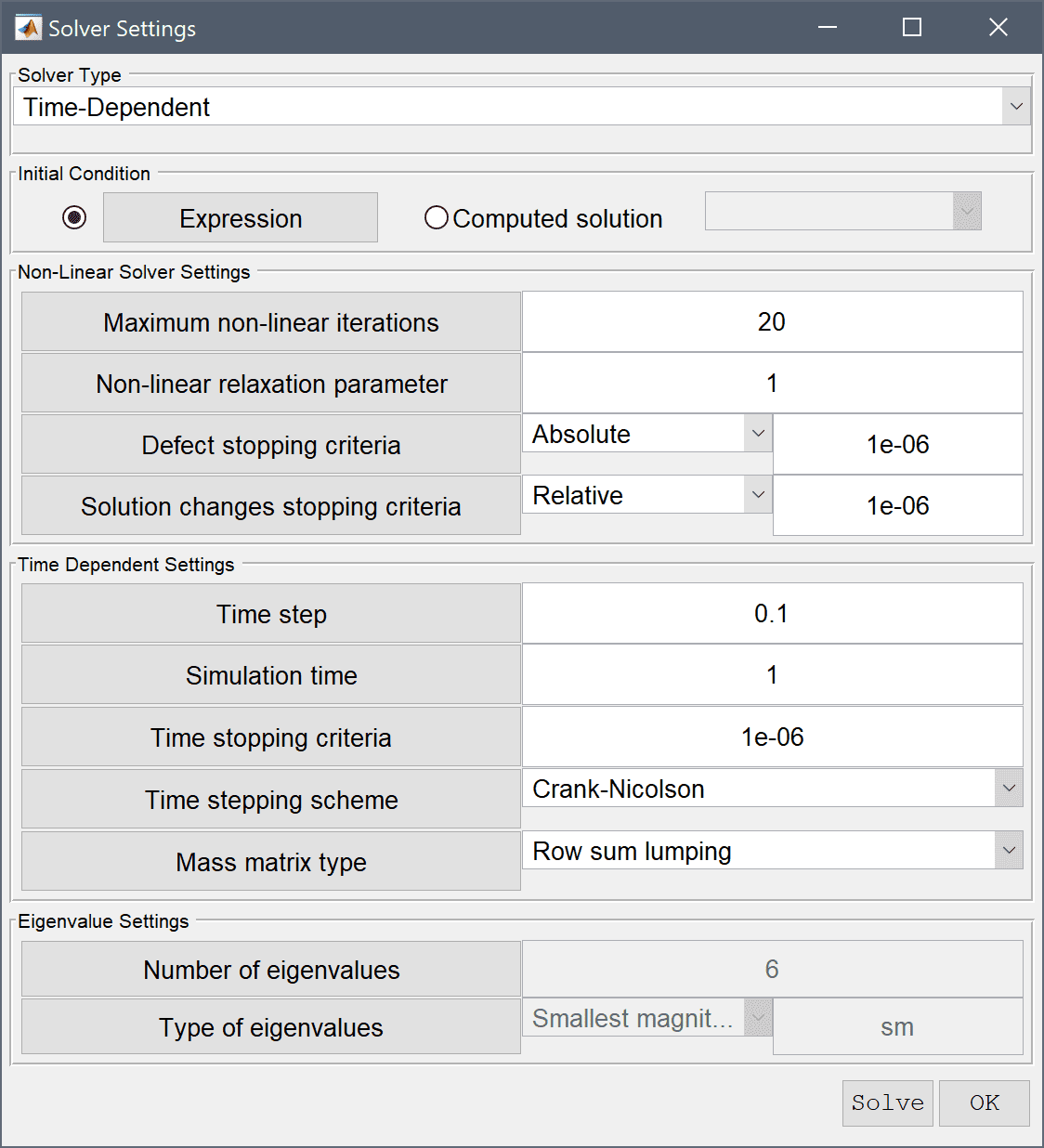
Press the Solve button.
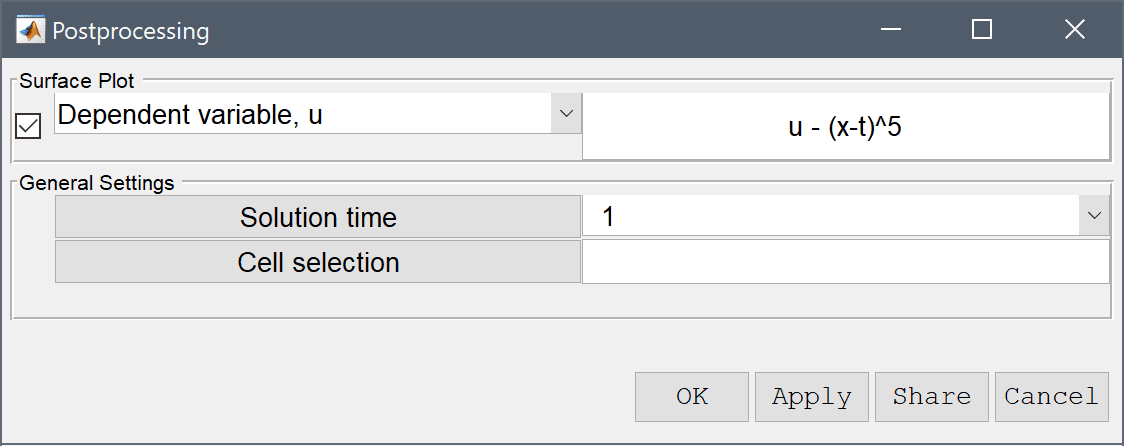
To visualize the difference between the computed and exact analytical solution, open the Plot Options and postprocessing settings dialog box and enter the expression u - (x-t)^5 in the edit field for the Surface Plot expression.
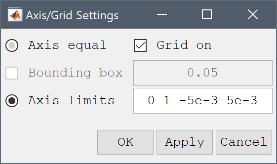
Enter 0 1 -5e-3 5e-3 into the edit field for the Axis limits (for the xmin, xmax, ymin, and ymax limits).
Press OK to finish and close the dialog box.
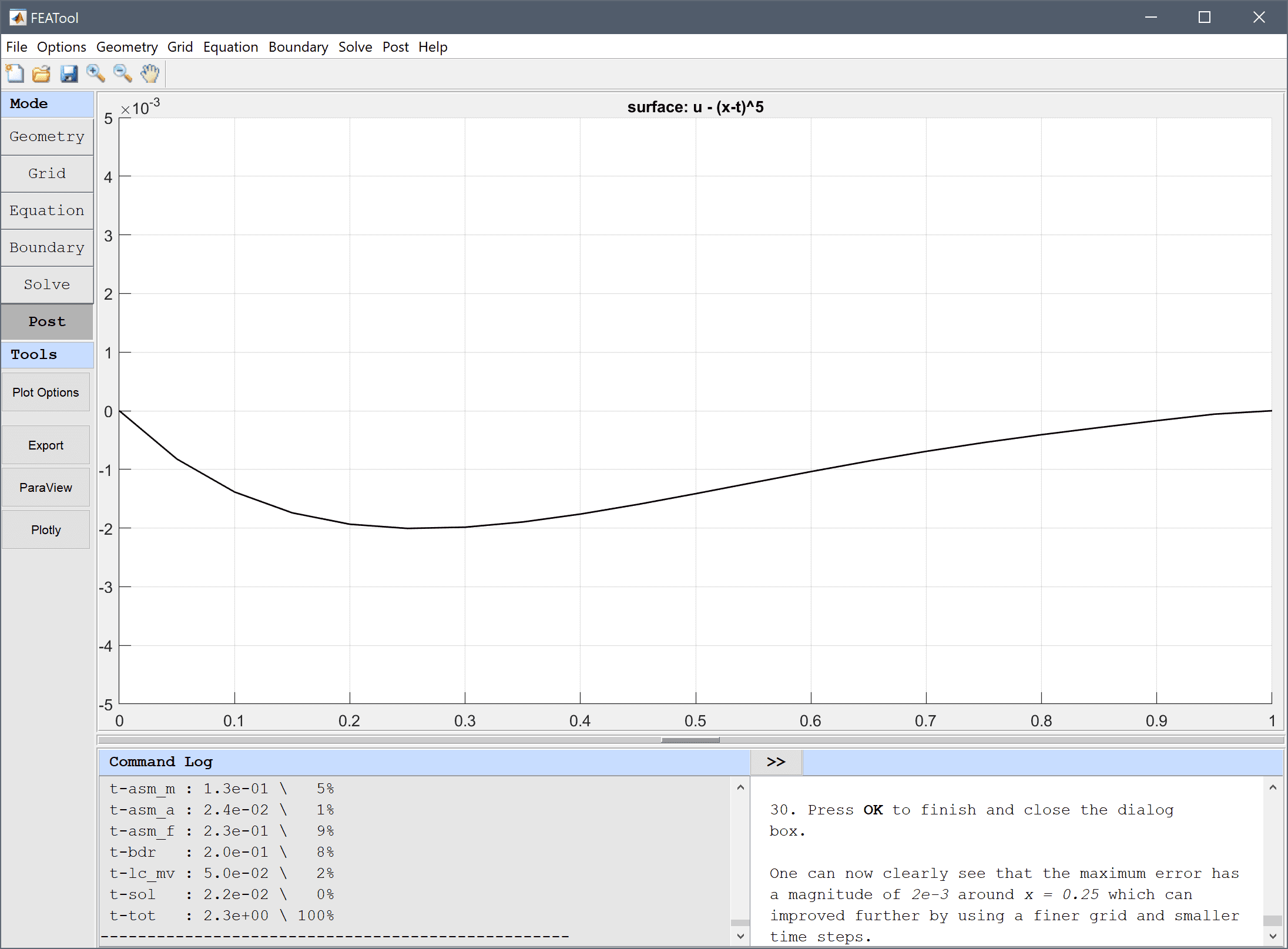
One can now clearly see that the maximum error has a magnitude of 0.002 around x = 0.25, which can be improved further by using a finer grid and smaller time steps.
The black-scholes equation classic pde model has now been completed and can be saved as a binary (.fea) model file, or exported as a programmable MATLAB m-script text file (available as the example ex_custom_equation1 script file), or GUI script (.fes) file.