FEATool is designed to be able to perform complex MATLAB multiphysics simulations in arbitrary dimensions (1D, 2D, and 3D). However, running full 3D simulations often requires a significant amount of computational resources in the form of memory and simulation time. It is therefore desirable to find simplifications to reduce simulations to two or even one dimension if possible.

Problems which feature cylindrical and rotationally symmetric geometries and solutions can be reduced to two dimensions through a cylindrical or axisymmetric coordinate transformation (also referred to 2.5D). A symmetry axis, usually r=0, is taken as reference around which the coordinates and PDE operators (gradient and divergence) are transformed. In this way the governing equations will be reduced to 2D while representing a rotationally symmetric three dimensional problem.

This example models fluid flow in a narrowing pipe section. The constriction of the pipe will accelerate the flow due to the venturi effect. As the fluid is assumed to be both laminar and isothermal the problem is governed by the incompressible Navier-Stokes equations. For scalar equations like the convection and diffusion, and heat transfer equations axisymmetric transformation simply results in a multiplication of the equation with the radial coordinate. In this case the vector valued equations results in additional terms compared to the usual Cartesian case

\[ \left\{\begin{aligned} r\rho\frac{\partial u}{\partial t} - r\mu(2\frac{\partial^2 u}{\partial r^2} + \frac{\partial^2 u}{\partial z^2} + \frac{\partial^2 v}{\partial r\partial z}) + r\rho(u\frac{\partial u}{\partial r} + v\frac{\partial u}{\partial z}) - 2\mu\frac{\partial u}{\partial r} + 2\mu\frac{u}{r} + r\frac{\partial p}{\partial r} &= 0 \\ r\rho\frac{\partial v}{\partial t} - r\mu( \frac{\partial^2 v}{\partial r^2} + \frac{\partial^2 u}{\partial z\partial r} + 2\frac{\partial^2 v}{\partial z^2}) + r\rho(u\frac{\partial v}{\partial r} + v\frac{\partial v}{\partial z}) - \mu\frac{\partial u}{\partial z} -\mu\frac{\partial v}{\partial r} + r\frac{\partial p}{\partial z} &= 0 \\ u + r\frac{\partial u}{\partial r} + r\frac{\partial v}{\partial z} &= 0 \end{aligned}\right. \]

In addition to modifying the equations an appropriate boundary condition for the symmetry boundary must be chosen. A homogeneous Neumann insulation/symmetry condition is typically employed for scalar equations, but in the case of fluid flow a slip condition preventing any radial velocity u(r=0) while allowing axial velocity is appropriate.

The geometry of the problem considers a 2:1 constriction with an initial pipe diameter of d = 2 m. The inlet velocity is assumed to be uniform v_in = v(z=0) = 1 m/s and the fluid has a density of ρ = 1 kg/m³ and viscosity µ = 0.05 kg/ms. This gives a Reynolds number of Re = ρ·v·d/µ = 40, which should result in laminar flow with a parabolic outflow profile.

Tutorial

How to set up and solve the axisymmetric flow problem with the FEATool Graphical User Interface (GUI) is described in the following. Alternatively, this tutorial example can also be automatically run by selecting it from the File > Model Examples and Tutorials > Quickstart menu, or viewed as a video tutorial. Note that the CFDTool interface differ slightly from the FEATool Multiphysics instructions described in the following.

Although FEATool features pre-defined physics modes for axisymmetric coordinate systems, this example shows how it is possible to use the edit equations feature to modify the built-in equations and accommodate custom equations.

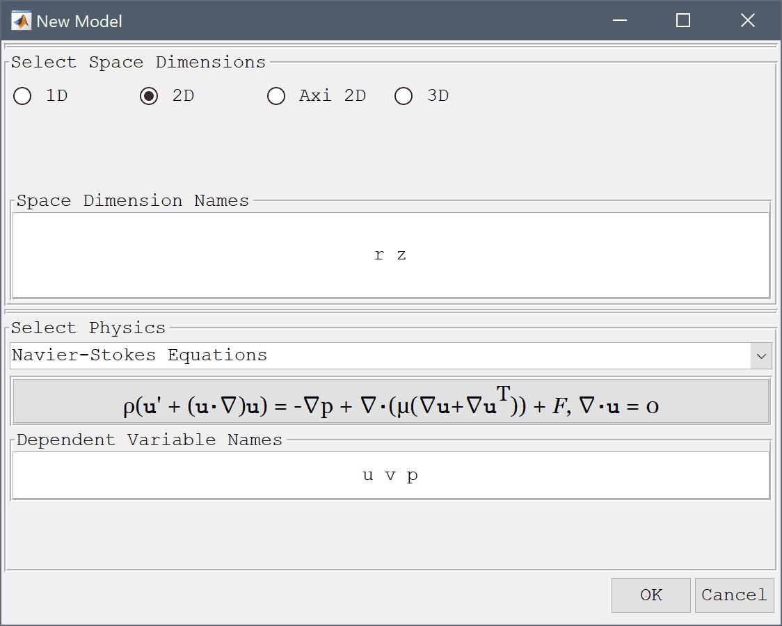
Start MATLAB and launch FEATool by clicking on the corresponding icon in the MATLAB Add-Ons toolbar (or type featool on the command line from the installation directory when not using FEATool as an installed toolbox).
To start a new model click the New Model toolbar button, or select New Model... from the File menu.

Click on the 2D Space Dimension selection button in the New Model dialog box, and select Navier-Stokes Equations from the Select Physics drop-down list (note that the Cartesian two dimensional equations will be manually modified in this example instead of using the pre-defined axisymmetric physics mode). Change the space dimension names to r and z, but leave the dependent variable names to their default values. Finish the physics selection and close the dialog box by clicking on the OK button. (Note that for CFDTool the physics selection is done in the Equation settings dialog box.)

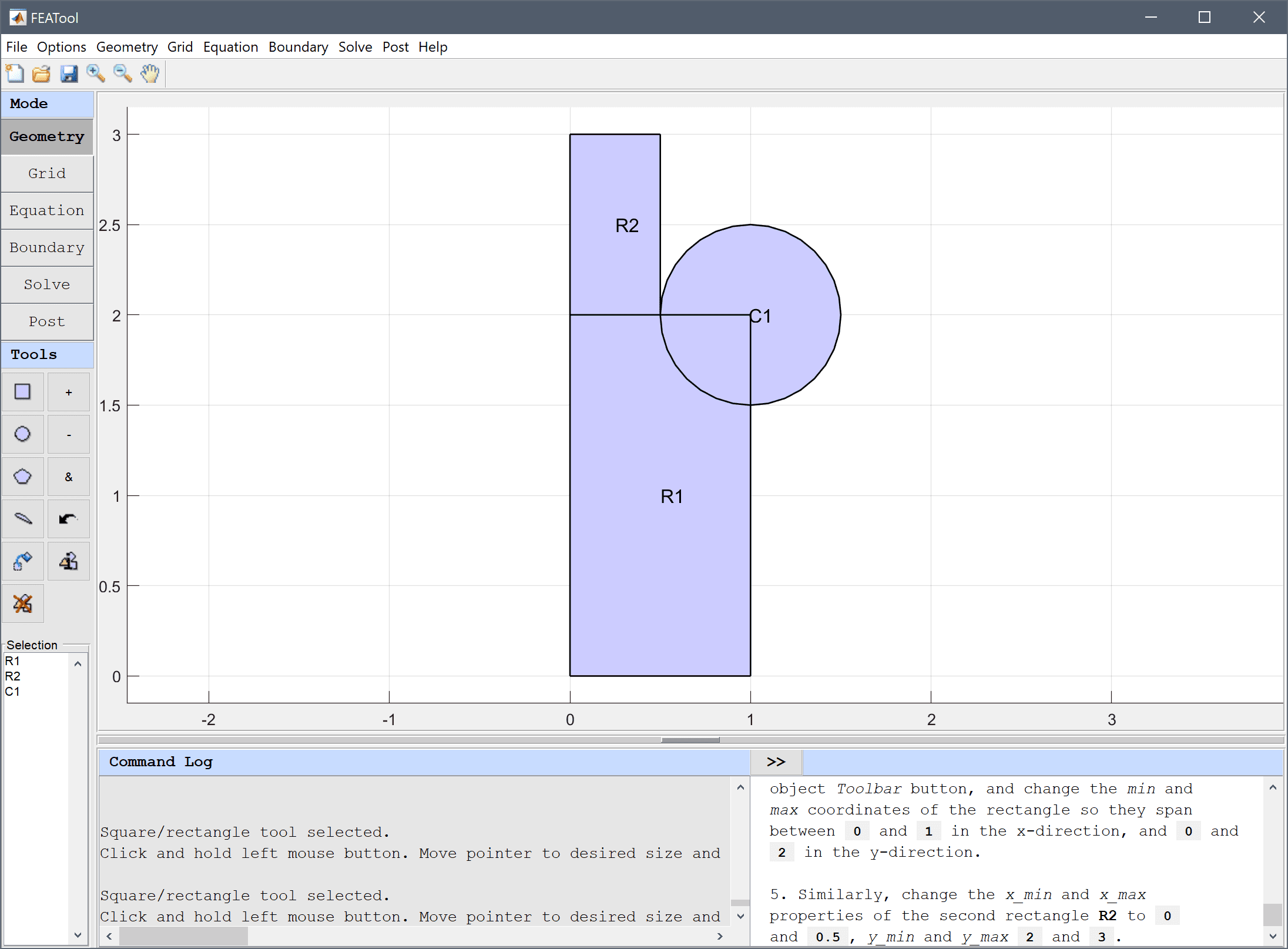
The geometry of the pipe cross section can be created by making 1 x 2 and 0.5 x 1 rectangles aligned with the (r = 0) symmetry axis, and also a circle with radius 0.5 centered at (1, 2), and finally subtracting the circle from the joined rectangles.

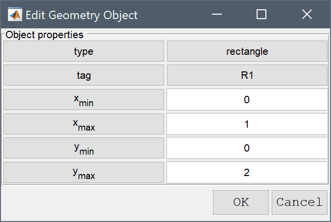
To create a rectangle, first click on the Create square/rectangle Toolbar button. Then left click in the main plot axes window, and hold down the mouse button. Move the mouse pointer to draw the shape outline, and release the button to finalize the shape.
The geometry object properties must now be edited to set the correct size and position of the rectangle. To do this, click on the rectangle R1 to select it which highlights it in red. Then click on the Inspect/edit selected geometry object Toolbar button, and change the min and max coordinates of the rectangle so they span between 0 and 1 in the x-direction, and 0 and 2 in the y-direction.
Similarly, change the x_min and x_max properties of the second rectangle R2 to 0 and 0.5, and y_min and y_max to 2 and 3.
To create the combined geometry, select Combine Objects... from the Geometry menu. Enter the formula R1 + R2 - C1 in the edit field of the Combine Geometry Objects dialog box and press OK.
Switch to Grid mode by clicking on the corresponding Mode Toolbar button.

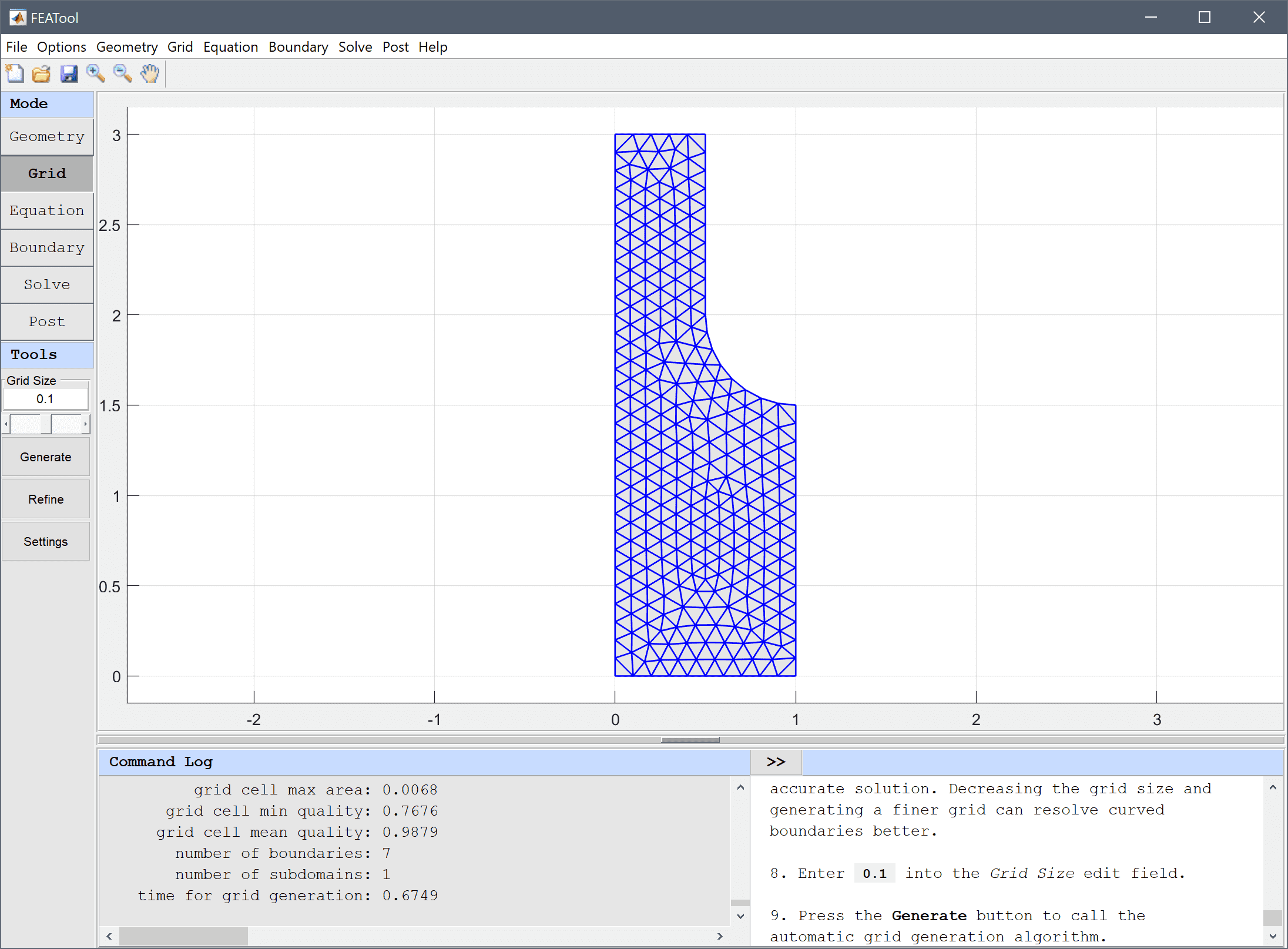
The default grid may be too coarse to ensure an accurate solution. Decreasing the grid size and generating a finer grid can resolve curved boundaries better.

Enter 0.1 into the Grid Size edit field and press the Generate button to call the automatic grid generation algorithm.
Switch to Equation mode by clicking on the corresponding Mode Toolbar button.
Equation and material coefficients are specified in Equation/Subdomain mode. In the Equation Settings dialog box enter 1 for the density, and 5e-2 for the viscosity. (Note that the Equation Settings dialog box may look different for CFDTool.)

Note that FEATool can work with any unit system, and it is up to the user to use consistent units for geometry dimensions, material, equation, and boundary coefficients.

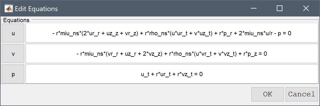
The equations must now be changed from the Cartesian to a axisymmetric/cylindrical coordinate system. To do this, press the edit button next to the equation description. This will bring up the equation editing dialog box where the defined partial differential equations can be inspected and edited. Change the equations according to the following.
Enter - r*miu_ns*(2*ur_r + uz_z + vr_z) + r*rho_ns*(u*ur_t + v*uz_t) + r*p_r + 2*miu_ns*u/r - p = 0 into the Equation for u edit field.
Enter - r*miu_ns*(vr_r + uz_r + 2*vz_z) + r*rho_ns*(u*vr_t + v*vz_t) + r*p_z = 0 into the Equation for v edit field.
Enter u_t + r*ur_t + r*vz_t = 0 into the Equation for p edit field.
Also select the (P2P1/Q2Q1) second order conforming Stokes element finite element discretization for higher accuracy, and to avoid having to reformulate the stabilization terms.
Press OK to finish with the equation editing and coefficient specifications.

Boundary conditions are defined in Boundary Mode and describes how the model interacts with the external environment.

Switch to boundary condition specification mode by clicking on Boundary the Mode Toolbar button. In the Boundary Settings dialog box, first choose all boundaries in the left hand side Boundaries list box and select the Wall/no-slip boundary condition from the drop-down menu. Now select the lower inflow boundary (number 1) in the left hand side Boundaries list box and select the Inlet/velocity boundary condition. Enter 1 in the edit field for the velocity v0 in the z-direction.
Select the top outflow boundary (number 5) and the Neutral outflow/stress boundary condition from the drop-down menu (alternatively, it is also possible prescribe a pressure at the outflow with the Outflow/pressure condition).
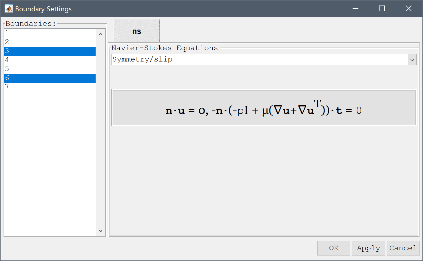
Lastly, select the left side boundaries on the symmetry axis (numbers 3 and 6), and select the Symmetry/slip boundary condition from the drop-down menu. This will prevent flow in the radial direction while allowing it in the axial direction. Finish the boundary condition specification by clicking the OK button.
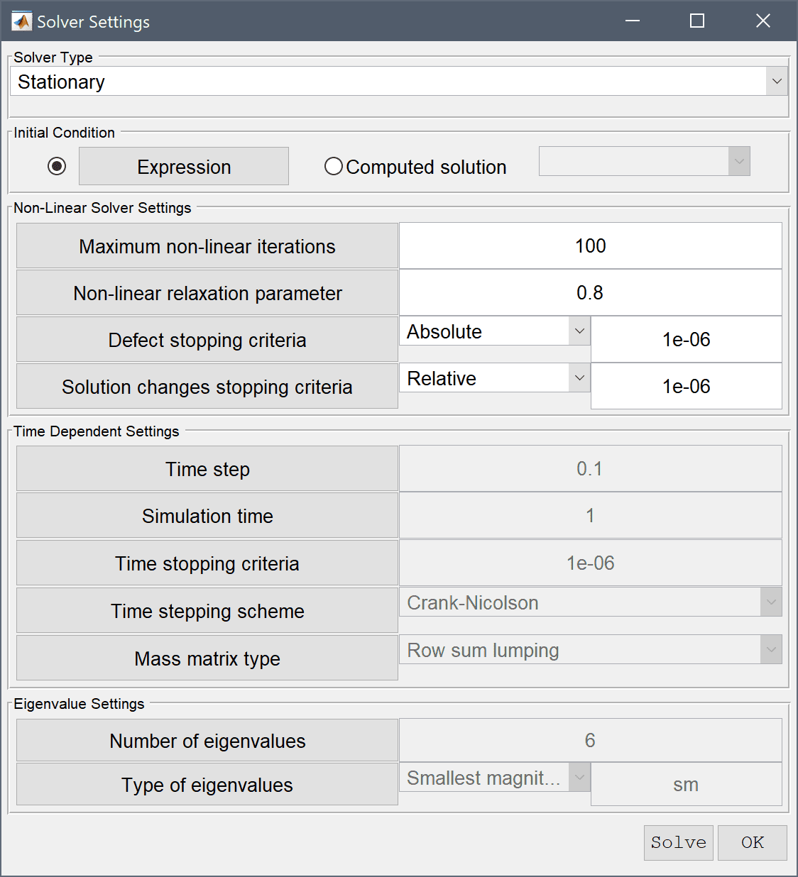
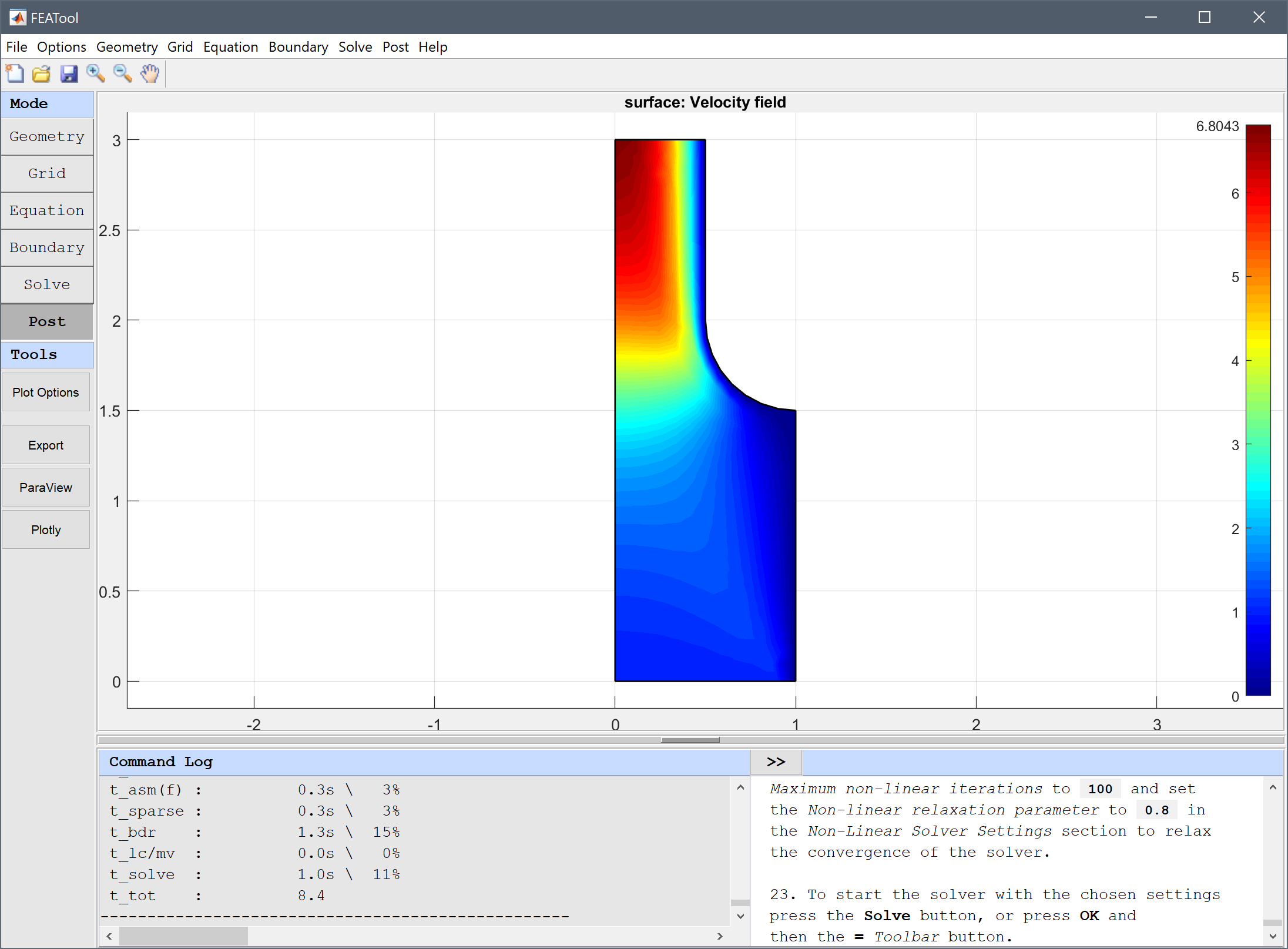
Now that the problem has been defined, press the Solve Mode Toolbar button to switch to solve mode, and press the Settings button to open the Solver Settings dialog box.
In the Solver Settings dialog box increase the Maximum non-linear iterations to 100, and set the Non-linear relaxation parameter to 0.8 in the Non-Linear Solver Settings section to relax the convergence of the solver.
To start the solver with the chosen settings press the Solve button, or press OK and then the = Toolbar button.

After the problem has been solved FEATool will automatically switch to postprocessing mode and display the computed velocity field, which clearly shows how the flow is significantly accelerated by the pipe constriction.

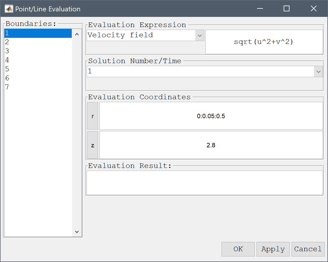
Cross sections of expressions such as the velocity profile can be plotted by using the Point/Line Evaluation... feature from the Post menu.

Select Point/Line Evaluation... from the Post menu.
Enter the evaluation coordinates 0:0.05:0.5 and 2.8 in the r and z-directions, respectively. These expressions give vectors of coordinates points to evaluate. Press Apply or OK to create a new figure with the cross section plot.

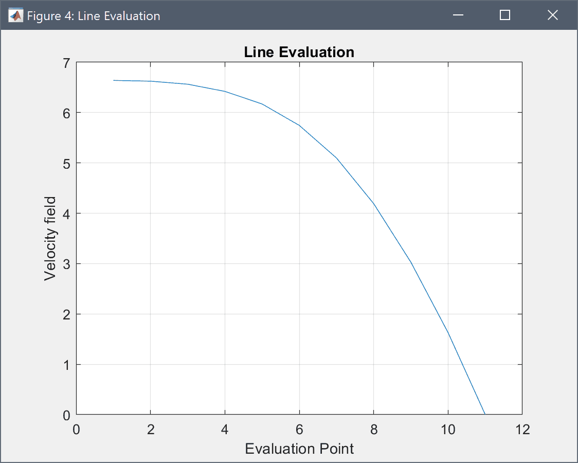
From the cross section plot one can see that the velocity profile close to the outlet, at z = 2.8, is starting to shift from parabolic to a more square profile indicating a higher flow rate. This also suggests that one might need to study a longer outflow section to allow for a fully developed parabolic laminar flow profile.

The axisymmetric fluid flow fluid dynamics model has now been completed and can be saved as a binary (.fea) model file, or exported as a programmable MATLAB m-script text file (available as the example ex_navierstokes8 script file), or GUI script (.fes) file.

CLI Postprocessing

To visualize the full 3D solution the model data can be exported to the MATLAB command line interface (CLI) console with the Export Model Data Struct to MATLAB option from the File menu. The postrevolve and postplot functions can then be applied to revolve and visualize the data, for example

fea_revolved = postrevolve( fea, 24, 0.75 );

postplot( fea_revolved, 'surfexpr', 'sqrt(u^2+v^2)', ...
          'parent', figure, 'axis', 'off', 'colorbar', 'off' )
view(65, 18)

Tutorial

CLI Postprocessing

Video