|
FEATool Multiphysics
v1.16.5
Finite Element Analysis Toolbox
|
|
FEATool Multiphysics
v1.16.5
Finite Element Analysis Toolbox
|
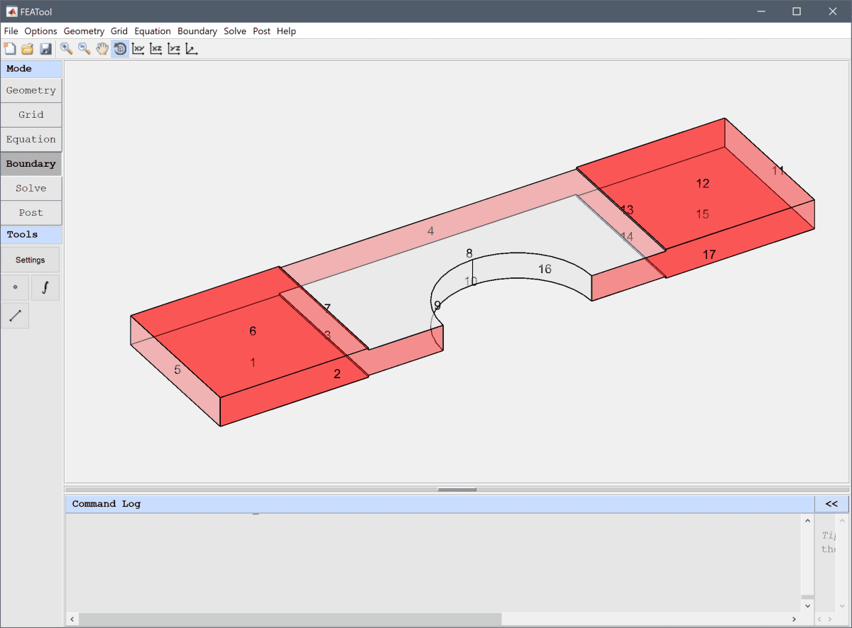
This model simulates how the flow of cool airflow is heated while moving through a tube-fin heat exchanger. Due to several symmetry planes only a small section of the heat exchanger geometry actually needs to be simulated, as illustrated in the following image.

This model illustrates the multi-solver simulation process for a coupled tube and fin heat exchanger. The flow field is first solved for using the OpenFOAM CFD solver, after which the temperature field is computed with the built-in FEA solver (using the known flow field as a input to the heat equation).
The process splits and separates the equations, effectively turning a one-way coupled model to a two step solution process with two sequential problems. This allows for significant savings in computational time and resources, since the best and most efficient physics solvers can be used for each individual sub-problem.
This model is available as an automated tutorial by selecting Model Examples and Tutorials... > Multiphysics > Multi-Simulation Heat Exchanger from the File menu, viewed as a video tutorial, or alternatively, follow the step-by-step instructions below. (Note that the external OpenFOAM solver needs to be installed for this model to run correctly.)
Press OK to finish the physics mode selection.
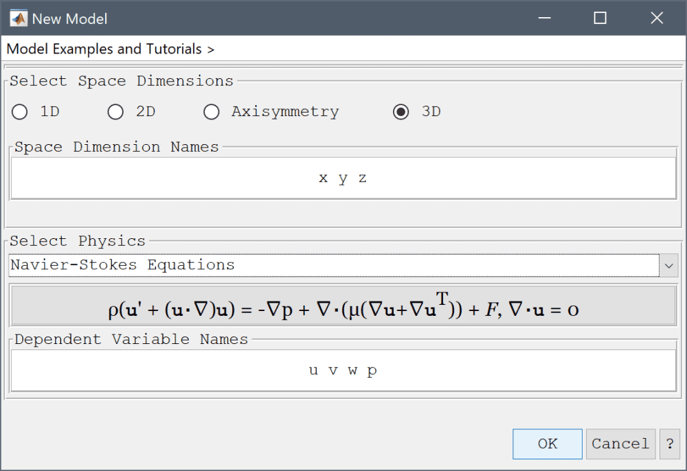
A heat transfer physics mode for the temperature field will be added and coupled later, after the flow field has been computed.
By utilizing the symmetry in the y and z directions the computational domain of the airflow can be significantly reduced to a slice between two fins and one tube. The resulting geometry can be constructed by subtracting the fins and a cylinder from a block. The first step is to create the main block for the interior of the domain.
20 into the xmax edit field.5 into the ymax edit field.Then create a cylinder and subtract it from the block.
10 0 0 into the edit field for the center of the cylinder.2.5 into the edit fields for both radius1 and radius2.0 0 1 into the axis edit field.Create the lower fin, and then make a copy with a z-translation to move it to the upper side.
5 into the xmin edit field.15 into the xmax edit field.5 into the ymax edit field.0.0625 into the zmax edit field.1 into the Number of copies to make edit field.0 0 0.9375 into the Displacement vector (x, y, and z-components) edit field.Lastly, remove the two fins using the geometry formula CS1 - B2 - B3.
CS1-B2-B3 into the Geometry Formula edit field.Press OK to finish and close the dialog box. The completed geometry should then look like the following.
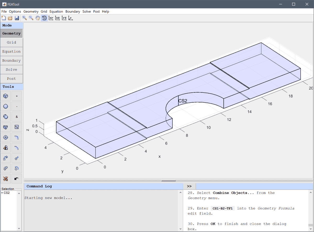
Generate a grid with the maximum target mesh size set to 0.2. Although this is a rather coarse mesh, it saves computational time and is good enough for demonstration purposes and as a first study.
0.2 into the Grid Size edit field.Press the Generate button to call the grid generation algorithm.

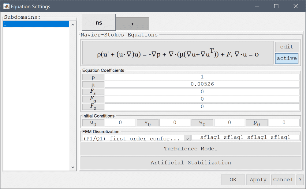
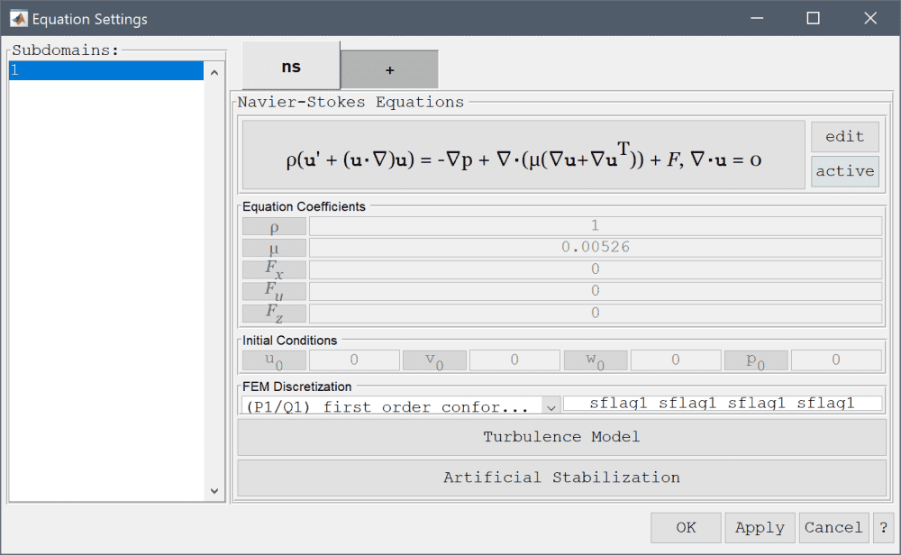
Enter a non-dimensionalized unit density of 1, and a viscosity of 0.00526. This is equivalent to a Reynolds number of 190 based on the distance between the heat exchanger fins.
1 into the Density edit field.Enter 0.00526 into the Viscosity edit field.
First, set the velocity on the inlet boundary in the x-direction to 1.
1 into the Velocity in x-direction edit field.Then select the Outflow/pressure condition for the outlet boundary.
Select the Wall/no-slip condition for the boundaries representing the fins and the cylinder (boundaries 3, 7-10, 13, 14, and 16).
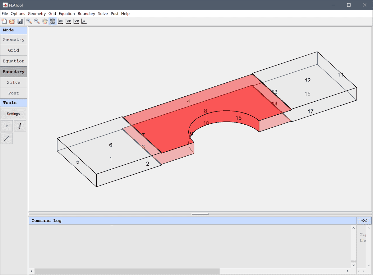
Finally, select the Symmetry/slip condition for the rest of the boundaries.
Select Symmetry/slip from the Navier-Stokes Equations drop-down menu.

The OpenFOAM CFD solver will be used to first solve for the flow field. Open the OpenFOAM solver settings dialog box and set the tolerance for convergence to 1e-4.
Enter 1e-4 into the Stopping criteria/tolerance for initial residuals edit field.
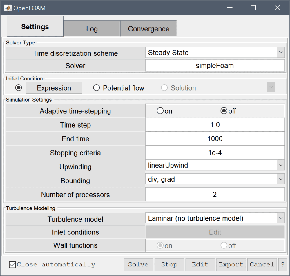
Press the Solve button to start the OpenFOAM solver. The view will switch to show the convergence process for the solution variables.
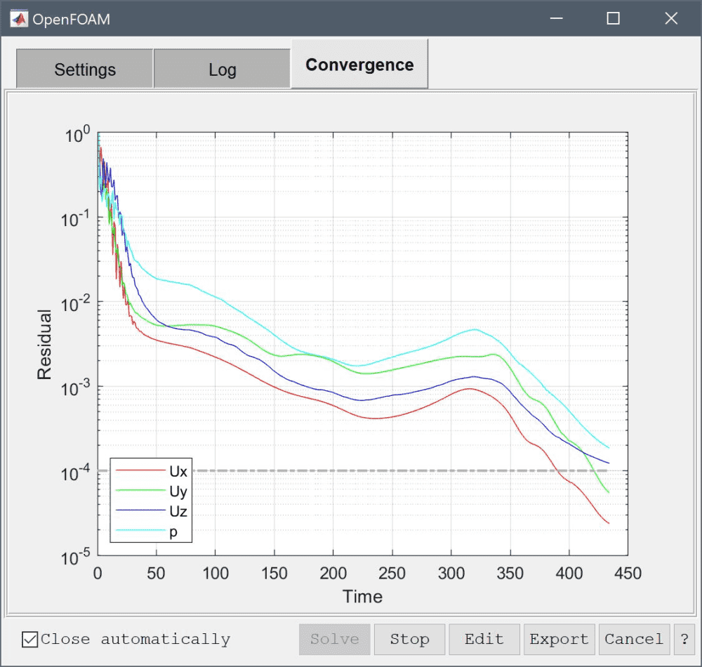
After the flow problem has been solved FEATool will automatically switch to postprocessing mode and display the resulting velocity field.
Open the Postprocessing settings dialog box and change from surface to slice plot to help see the interior of the flow field.
Press OK to plot and visualize the selected postprocessing options.

One can now clearly see that there is a large wake behind the cylinder, and how the fins create a very thin low velocity boundary layer.
To couple and study the temperature field, switch back to Equation mode and add a Heat Transfer physics mode to the model.
First deactivate the equation for the flow field by de-selecting the active button. This means that the flow variables will not be solved for and held constant, which saves computational effort. (Note that this decoupling is only possible for one-way coupled multiphysics problems. If the flow field and properties also depend on the temperature, both physics modes must be fully coupled and solved for together.)
Set the non-dimensionalized thermal conductivity to 3.76e-3, while leaving the density and heat capacity at their default unit values. This is equivalent to a Prandtl number of 1.4 (indicating a slight weighting toward convective transport).
3.76e-3 into the Thermal conductivity edit field.To couple the flow field to the convective terms for the temperature, enter the dependent variable names u, v, and w in the corresponding edit fields.
u into the Convection velocity in x-direction edit field.v into the Convection velocity in y-direction edit field.Enter w into the Convection velocity in z-direction edit field.

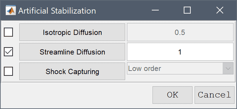
As this model is dominated by convective flow effects some amount of artificial and numerical stabilization is appropriate to add, which will ease convergence and smooth out oscillations.
Enter 1 into the Streamline diffusion tuning parameter edit field.
For the temperature boundary conditions set the inlet temperature to 0, and the surfaces of the surrounding fins and cylinder to 1.
0 into the Temperature edit field.1 into the Temperature edit field.For the outflow boundary select Convective flux/outflow.
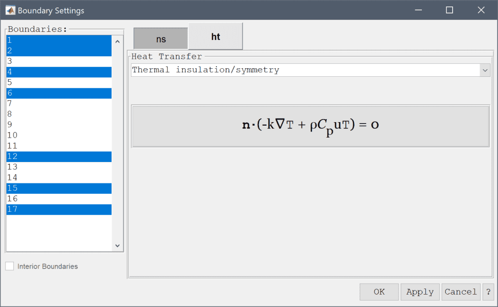
And finally select Thermal insulation/symmetry for the symmetry boundaries.
Select 1, 2, 4, 6, 12, 15, and 17 in the Boundaries list box.
Select Thermal insulation/symmetry from the Heat Transfer drop-down menu.
Press the ![]() Restart button to solve the problem for the temperature field using the already computed flow field (as the Navier-Stokes equations physics mode was deactivated earlier). (Do not use the usual = solve button, as this would clear the already computed flow field and instead re-compute the initial conditions.)
Restart button to solve the problem for the temperature field using the already computed flow field (as the Navier-Stokes equations physics mode was deactivated earlier). (Do not use the usual = solve button, as this would clear the already computed flow field and instead re-compute the initial conditions.)
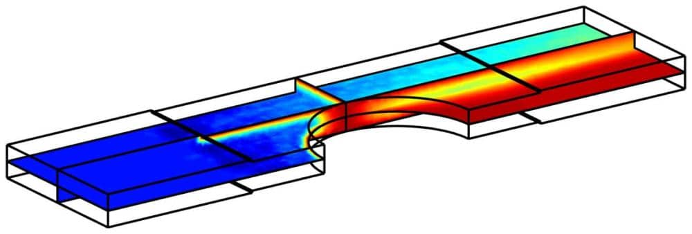
After the solution process is done the temperature field can now be plotted and visualized.
Press OK to plot and visualize the selected postprocessing options.

One can clearly see how the fluid is heated by both the cylinder and walls, and transported away in the direction of the flow.
The multi-simulation heat exchanger multiphysics model has now been completed and can be saved as a binary (.fea) model file, or exported as a programmable MATLAB m-script text file, or GUI script (.fes) file.
To visualize the full 3D solution the model data can be exported to the MATLAB command line interface (CLI) console with the Export Model Data Struct to MATLAB option from the File menu. The following advanced script can then be used to recreate the full model
% Create and plot full heat exchanger geometry.
geom.objects = {};
zoffset = 0;
for i=1:21
  tag = ['B',num2str(i)];
  gobj = gobj_block( [5], [15], [0], [40], [zoffset-0.0625], [zoffset+0.0625], tag );
  geom.objects{i} = gobj;
  zoffset = zoffset + 1;
end

yoffset = 0;
for i=1:4
  tag = ['C',num2str(i)];
  gobj = gobj_cylinder( [10 yoffset+5 -5], [2.5], [30], [0 0 1], tag );
  geom.objects = [ geom.objects, {gobj} ];
  yoffset = yoffset + 10;
end

fig = figure;
hold on
plotgeom( geom, 'parent', fig, 'labels', 'off' )

% Plot simulation data.
fea.grid.p(3,:) = fea.grid.p(3,:) + 10;
fea.grid.p(2,:) = fea.grid.p(2,:) + 5;
h = postplot(fea, 'parent', fig, 'sliceexpr', 'T', 'slicex', [], 'slicey', [], 'slicez', 10+0.3);
hp = findall(h,'type','patch');
delete(setdiff(h,hp))

pdata = get( hp, {'vertices', 'faces', 'facevertexcdata'} );
p = pdata{1};
for yoff=[10, 10, 10]
  p(:,2) = p(:,2) + yoff;
  patch( 'vertices', p, 'faces', pdata{2}, 'facevertexcdata', pdata{3},  'facecolor', 'interp', 'linestyle', 'none' );
end

p = pdata{1};
p(:,2) = 10 - p(:,2);
for yoff=[0, 10, 10, 10]
  p(:,2) = p(:,2) + yoff;
  patch( 'vertices', p, 'faces', pdata{2}, 'facevertexcdata', pdata{3},  'facecolor', 'interp', 'linestyle', 'none' );
end

% Offset fea data.
fea.grid.p(2,:) = fea.grid.p(2,:) + 10;
hfea = postplot( fea, 'parent', fig, 'streamexpr', {'u', 'v', 'w'} );

% Camera settings.
view(3)
axis off
alpha(0.05)
for i=length(geom.objects)-3:length(geom.objects)
  set(findall(0,'tag',['fea_geomp',num2str(i)]),'FaceAlpha',0.2)
end
set(findall(0,'tag','geom_slice'),'FaceAlpha',1)
set(hp,'FaceAlpha',1)
delete(findall(0,'type','light'))
camlight headlight