|
|
FEATool Multiphysics
v1.18.1
Finite Element Analysis Toolbox
|
|
|
FEATool Multiphysics
v1.18.1
Finite Element Analysis Toolbox
|
This classic double-slit experiment considers a planar and periodic oscillating wave, which hits and passes two narrow slits. Assuming the slits are narrow enough, the passing waves will bend and cause an interference pattern, while diffraction will attenuate the resulting off-axis amplitude.
In the example the Helmholtz equation is used to model the wave phenomena
\[ -( \frac{\partial^2 A}{\partial x^2} + \frac{\partial^2 A}{\partial y^2} ) - k^2 A = 0 \]
where A is the amplitude of the wave,and k the wave number (k = 2·π/λ).
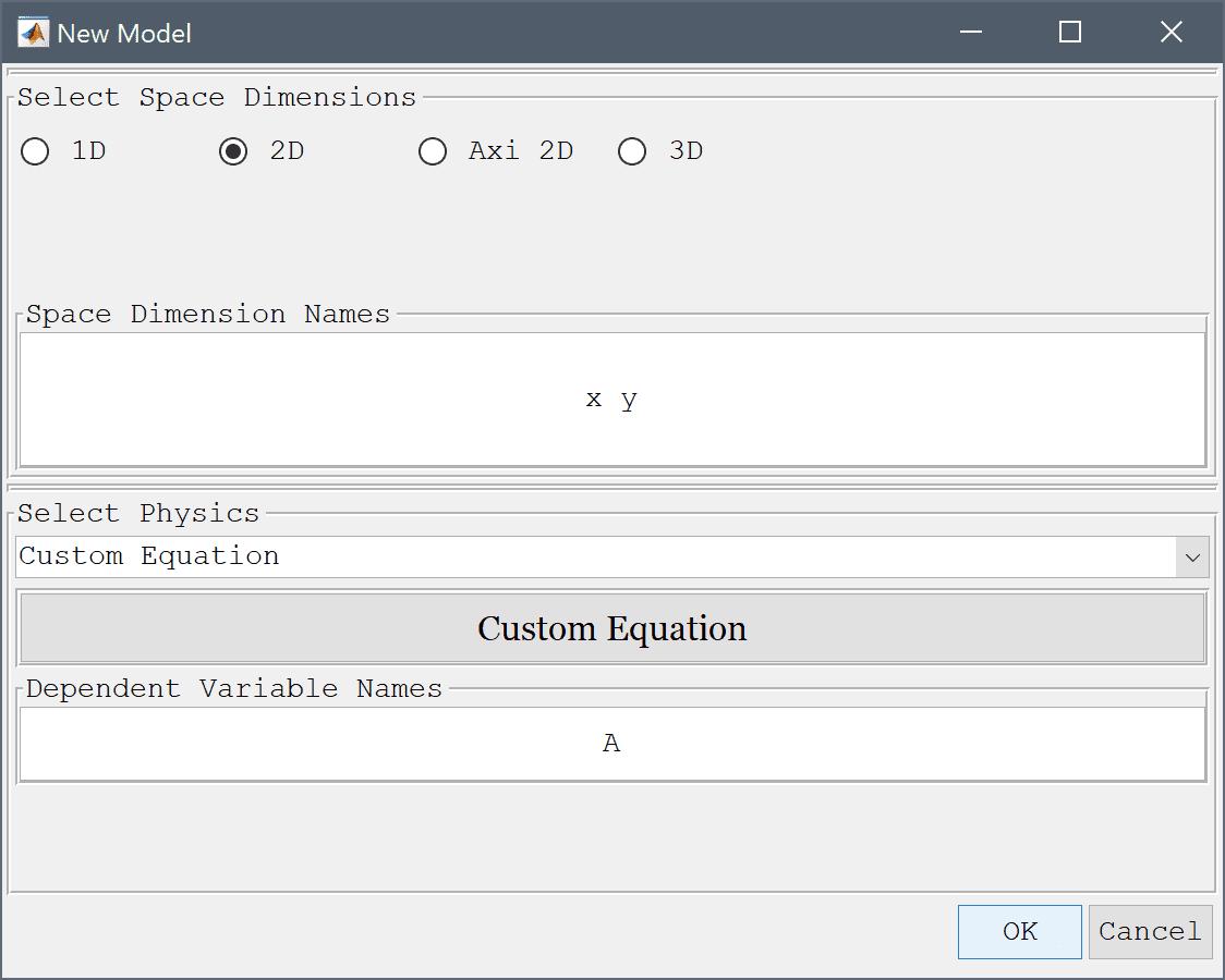
This model is available as an automated tutorial by selecting Model Examples and Tutorials... > Classic PDE > Interference and Diffraction from the File menu, viewed as a video tutorial, or alternatively, follow the step-by-step instructions below.
Enter A into the Dependent Variable Names edit field. This will represent the amplitude of the wave.
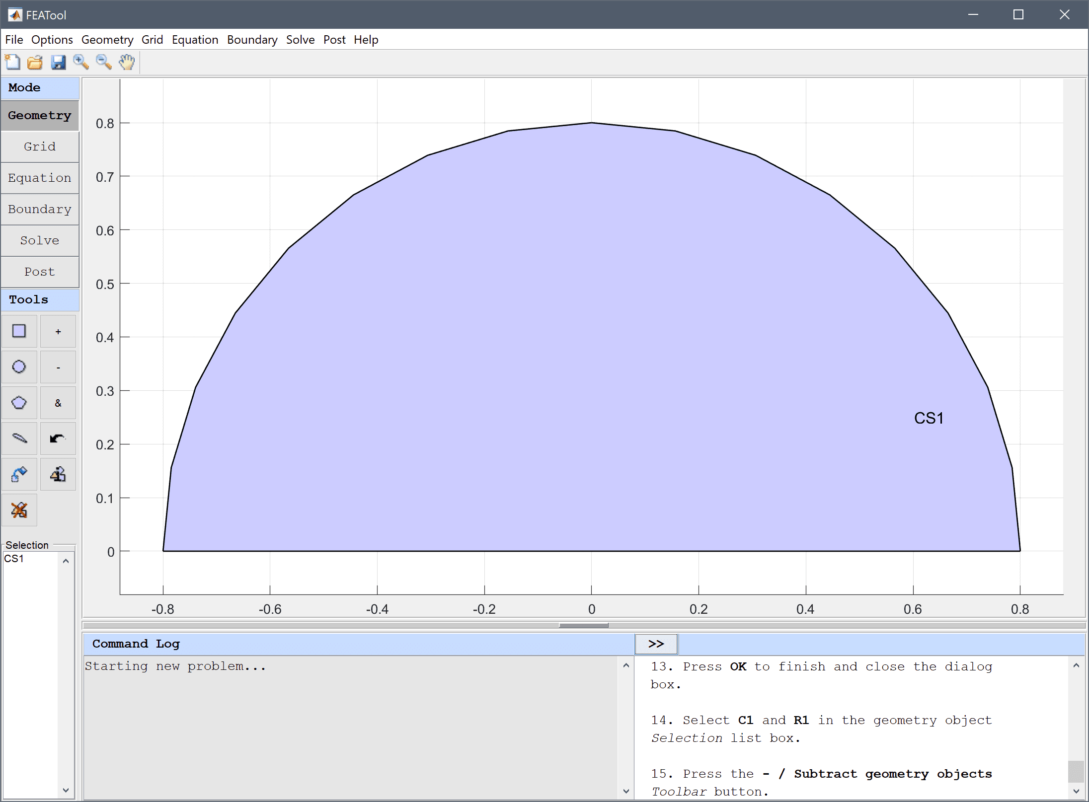
The geometry consists of two small rectangles, representing the slits, connected to a half circle domain. First create a circle centerd at the origin with radius 0.8.
0.8 into the radius edit field.Then create and subtract a rectangle from the lower half of the circle.
-0.8 into the xmin edit field.0.8 into the xmax edit field.-0.8 into the ymin edit field.0 into the ymax edit field.Press the - / Subtract geometry objects Toolbar button.
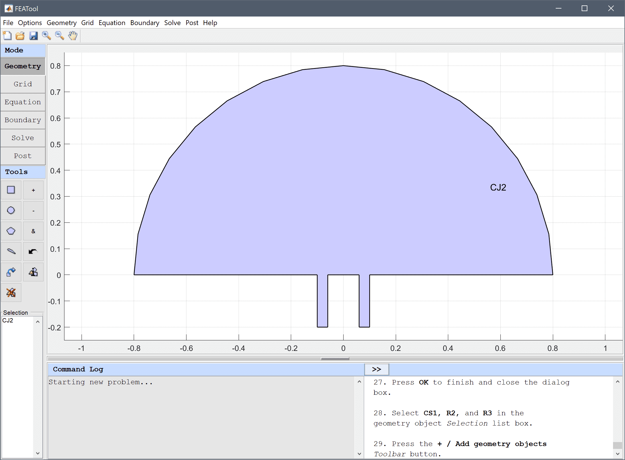
-0.08-0.02 into the xmin edit field.-0.08+0.02 into the xmax edit field.-0.2 into the ymin edit field.0 into the ymax edit field.0.08-0.02 into the xmin edit field.0.08+0.02 into the xmax edit field.-0.2 into the ymin edit field.0 into the ymax edit field.Press the + / Add geometry objects Toolbar button.
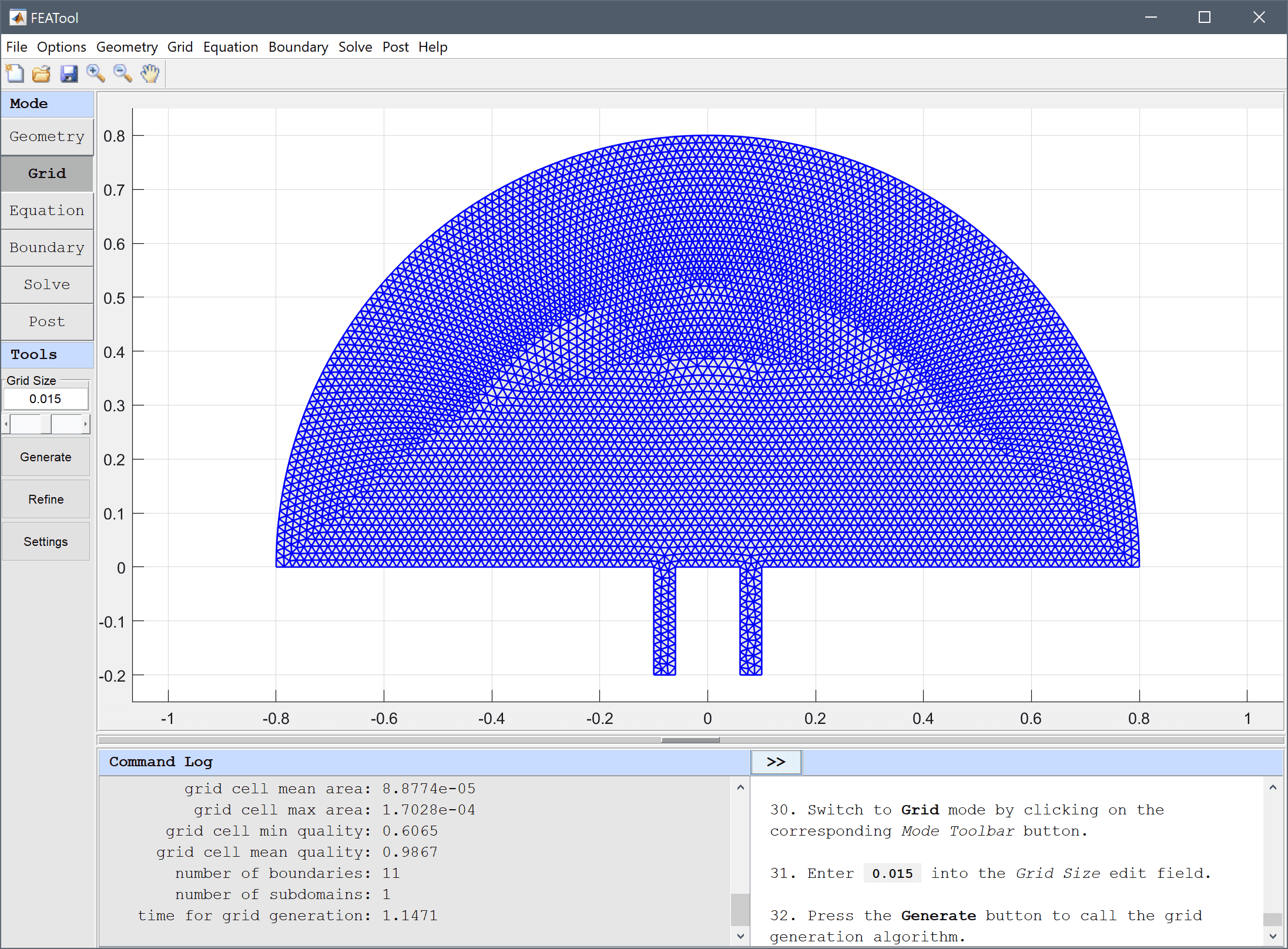
Enter 0.015 into the Grid Size edit field, and press the Generate button to call the grid generation algorithm.
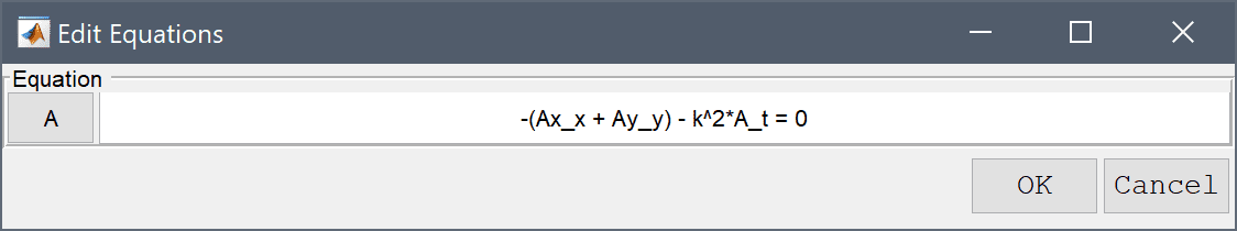
Enter -(Ax_x + Ay_y) - k^2*A_t = 0 into the Equation for A edit field.
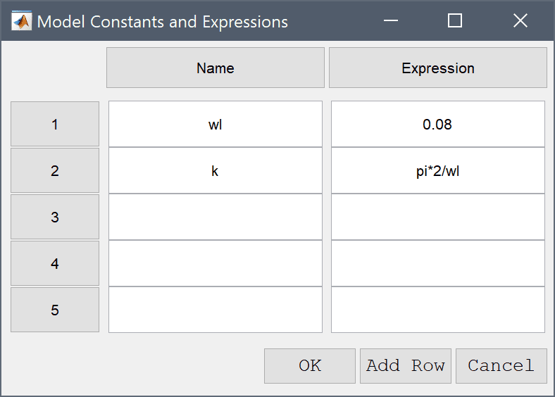
| Name | Expression |
|---|---|
| wl | 0.08 |
| k | pi*2/wl |
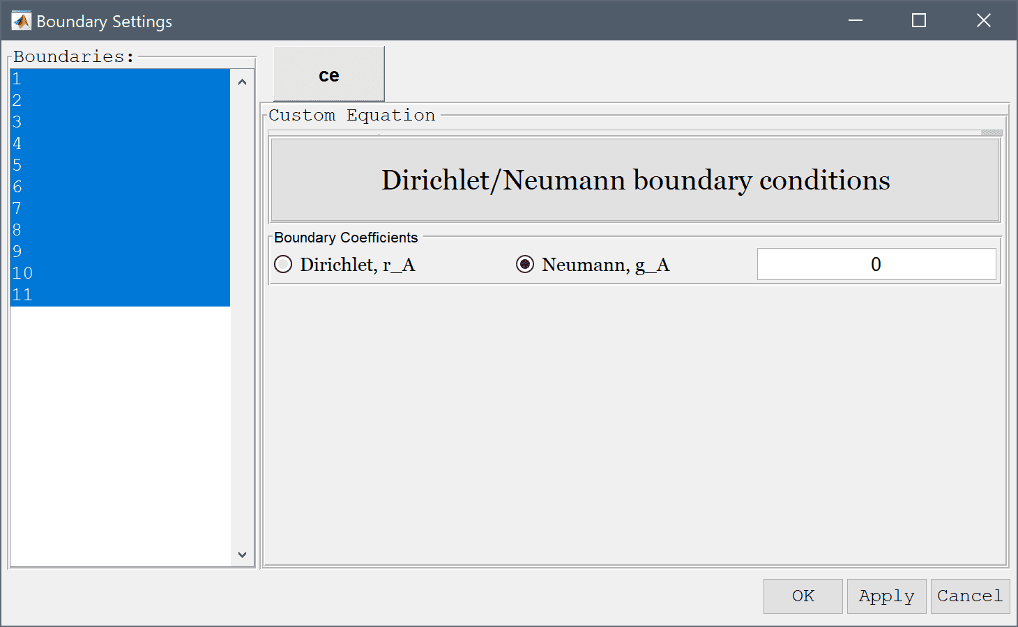
First set homogeneous Neumann conditions for all the boundaries.
Then select the Neumann, g_A radio button, and enter 0 into the Dirichlet/Neumann coefficient edit field.
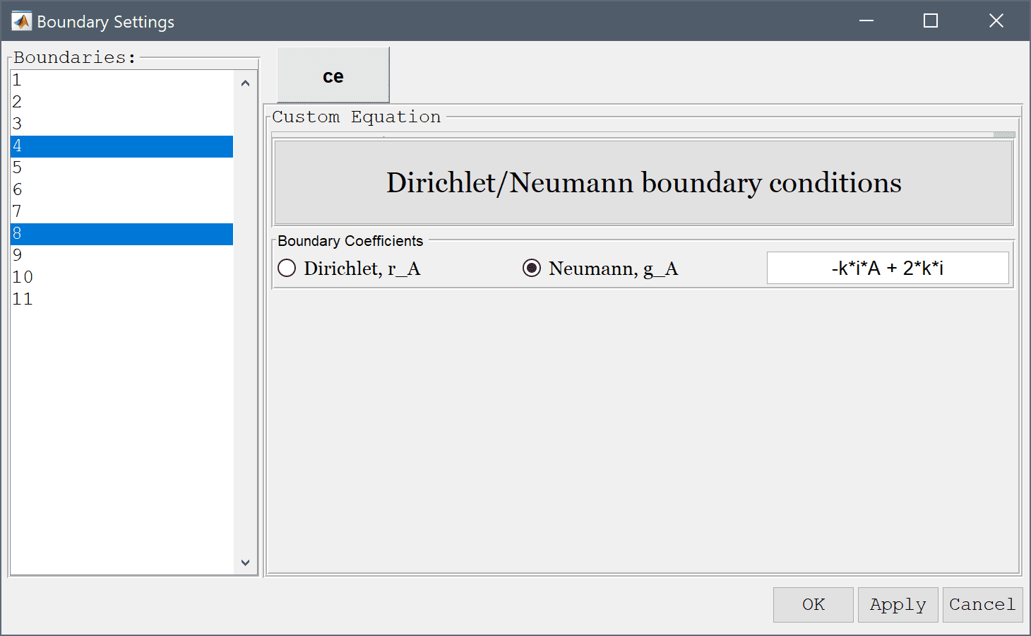
An incoming planar wave is present at the inlet, with the complex boundary condition n·∇(A) + k·i·A = 2·k·i, which can be implemented as a Neumann flux type boundary condition.
Select 3 and 7 in the Boundaries list box, and enter -k*i*A + 2*k*i into the Dirichlet/Neumann coefficient edit field.
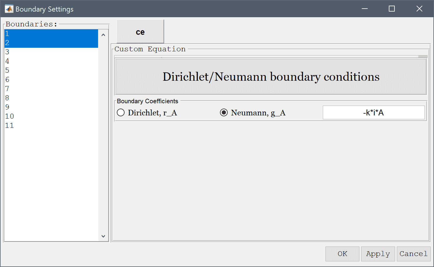
The outlet is assumed non-reflective and therefore n·∇(A) + k·i·A = 0.
Enter -k*i*A into the Dirichlet/Neumann coefficient edit field.
After the problem has been solved FEATool will automatically switch to postprocessing mode, and display the computed wave amplitude A. The interference pattern can clearly be seen, as the four distinct lines where the waves have been completely canceled out.
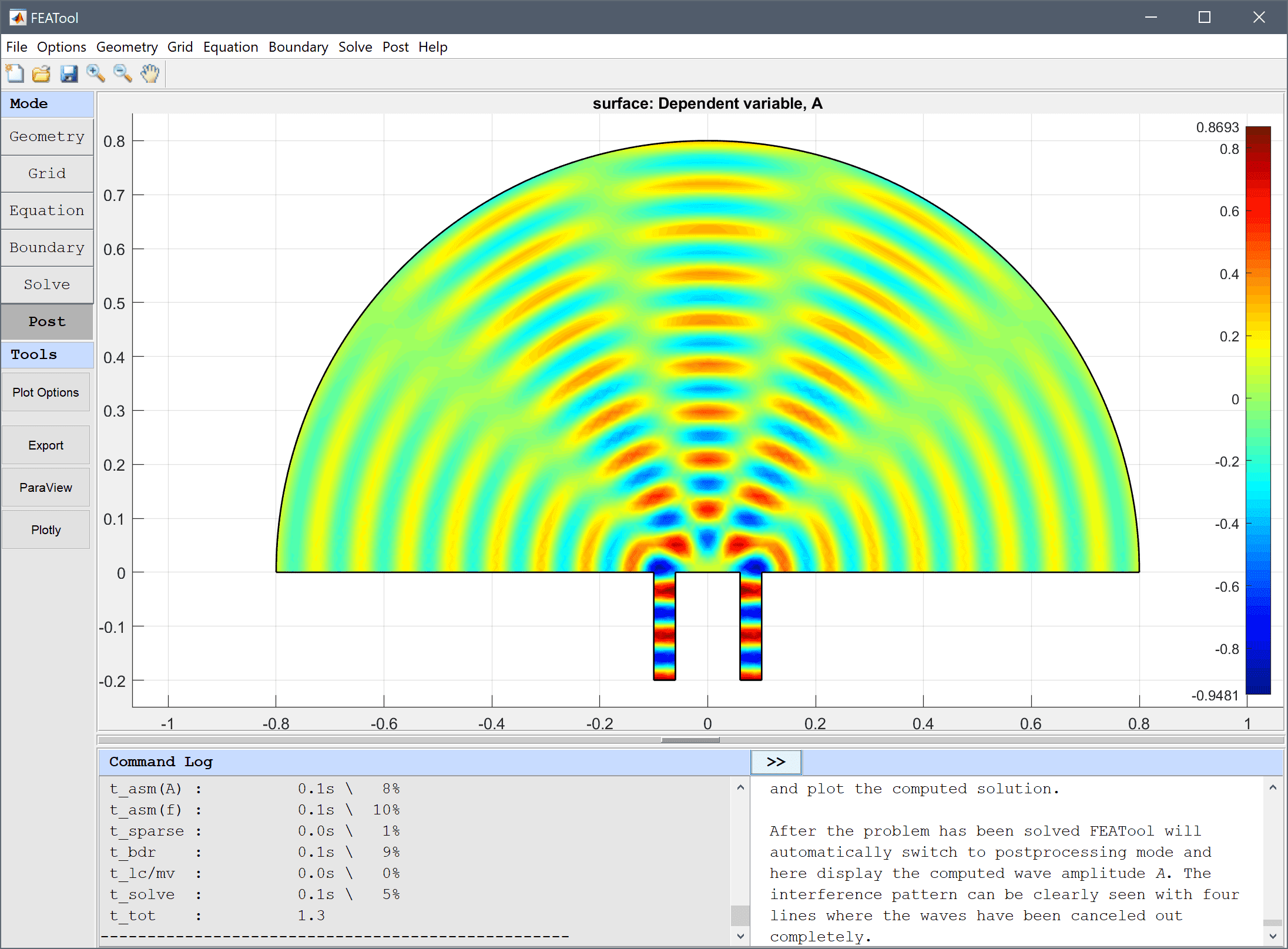
The Point/Line Evaluation tool can be used to visualize the interference and diffraction pattern at the boundary.
Select 10 and 11 in the Boundaries list box. This will automatically enter the corresponding boundary coordinates into the Evaluation Coordinates edit fields. Then press Apply or OK to finish and plot the amplitude curve.
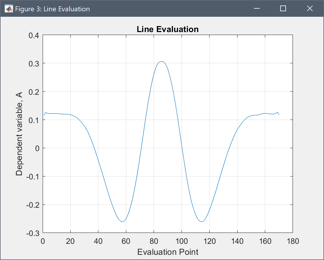
Even though the values for boundary 11 are plotted in reverse, one can clearly see the four intersections with the zero amplitude line. From theory the minima and maxima are given as sin(θ) = (n+½)λ/L and nλ/L, respectively (for n=0, ±1, etc where L is the distance between the slits), which here should be 0 and 30 degrees for the maxima, consistent with the results of the simulation.
The interference and diffraction custom equation model has now been completed and can be saved as a binary (.fea) model file, or exported as a programmable MATLAB m-script text file, or GUI script (.fes) file.