|
|
FEATool Multiphysics
v1.18.1
Finite Element Analysis Toolbox
|
|
|
FEATool Multiphysics
v1.18.1
Finite Element Analysis Toolbox
|
Flow over backwards facing steps are classic computational fluid dynamics test problems, and are often used for validation of simulation codes. This test case consists of studying how the flow field reacts to a sudden expansion in a channel. The expansion will cause a break in the flow and a recirculation or separation zone will form. To validate the results the computed length of the recirculation zone is compared with the experimental results of Pitz and Daily [1].
In this example the stationary incompressible Navier-Stokes equations are used to model the fluid with simulation parameters corresponding to a Reynolds number, Re = 18000. The flow is therefore fully turbulent, whereby a turbulence model closure must also be applied. Here the standard k-epsilon turbulence model is used which are available with both the OpenFOAM and SU2 CFD solver integrations built into FEATool Multiphysics.
This model is available as an automated tutorial by selecting Model Examples and Tutorials... > Fluid Dynamics > Turbulent Flow Over a Backwards Facing Step from the File menu, viewed as a video tutorial, or alternatively, follow the step-by-step instructions below. (Note that the external OpenFOAM solver needs to be installed for this model to run correctly.)
In this example variations in the z-direction are assumed to be negligible which enables using a planar 2D approximation, and saving computational cost compared to a full 3D simulation.
Press the 2D radio button and select the Navier-Stokes Equations physics mode from the Select Physics drop-down menu.
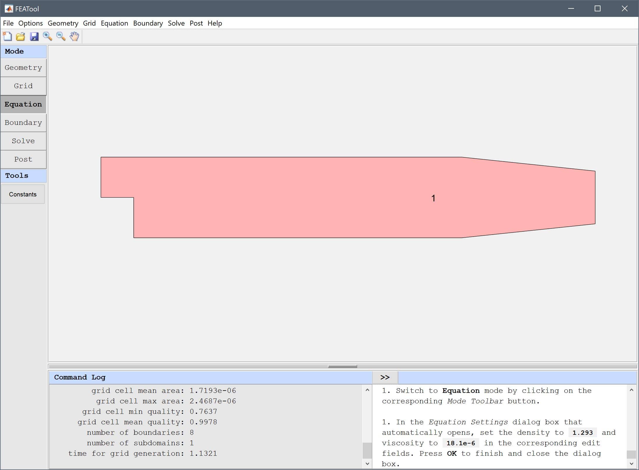
The backwards facing step geometry features a slightly tapered outflow region, which is easiest to create by directly specifying a polygon by coordinates.
| 1 | 2 | 3 | 4 | 5 | 6 | 7 | 8 | |
|---|---|---|---|---|---|---|---|---|
| x | -0.0206 | 0 | 0 | 0.206 | 0.29 | 0.29 | 0.206 | -0.0206 |
| y | 0 | 0 | -0.0254 | -0.0254 | -0.0166 | 0.0166 | 0.0254 | 0.0254 |
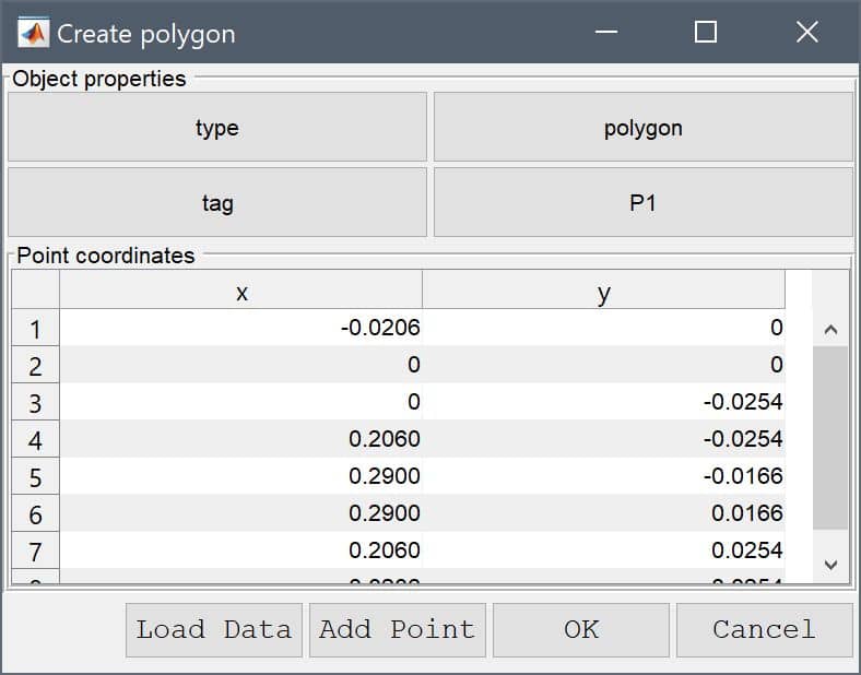
Press OK to finish and close the dialog box. The geometry should now look like the following.
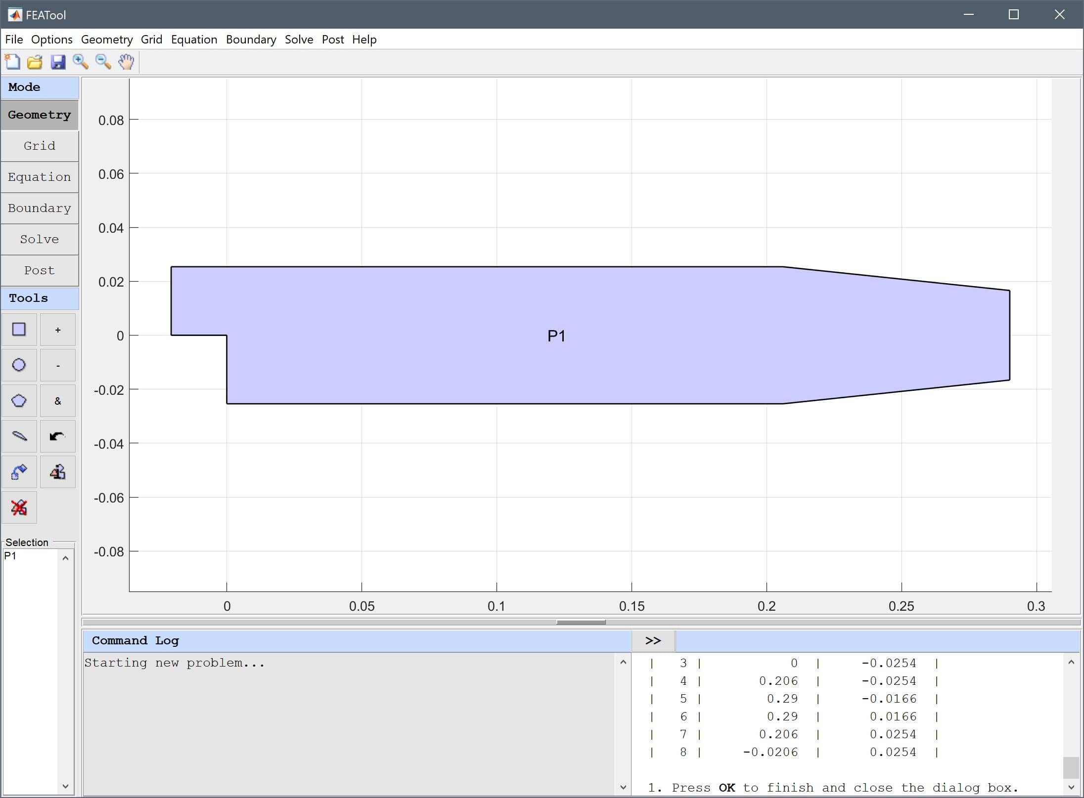
The dimensions are here given in meters. However, note that the toolbox works with any unit system, and it is up to the user to choose consistent units for geometry dimensions, material, equation, and boundary coefficients.
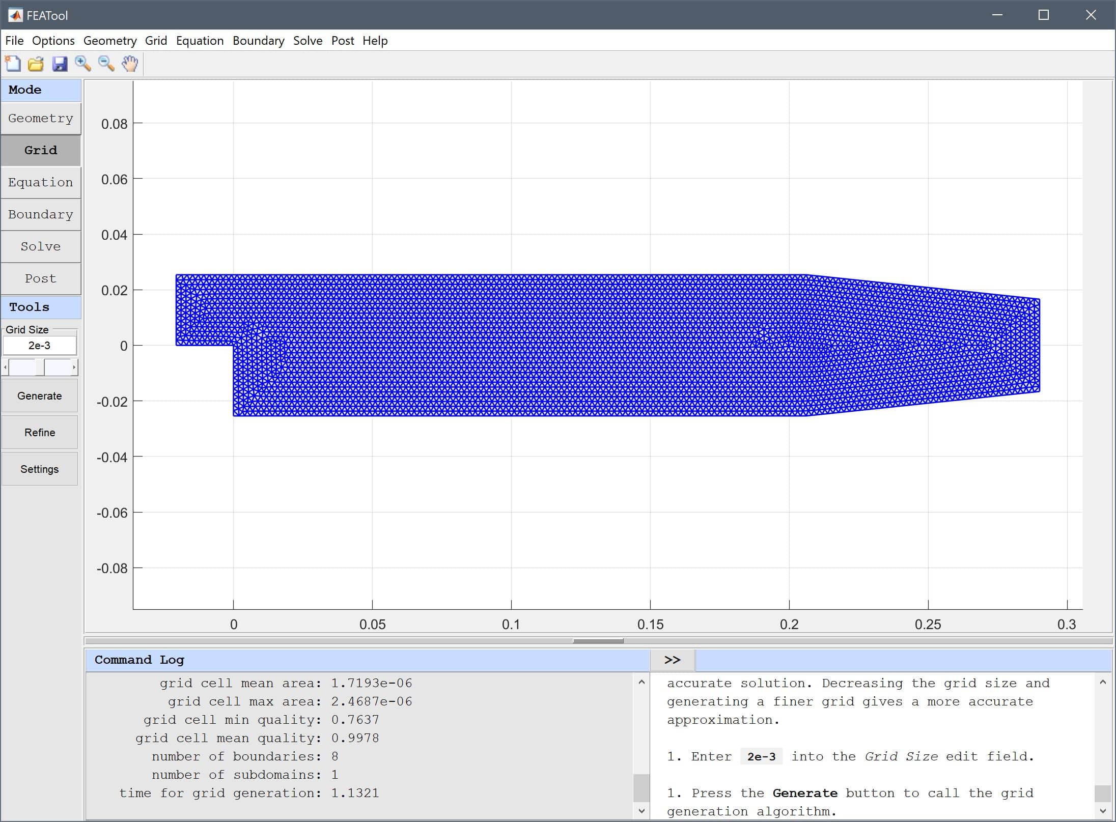
For turbulent flows it is particularly important to ensure a fine resolution near walls, due to viscous boundary layers which feature steep gradients.
The default grid will be too coarse to ensure an accurate solution. To create a finer grid, enter 0.002 into the Grid Size edit field, and press the Generate button.
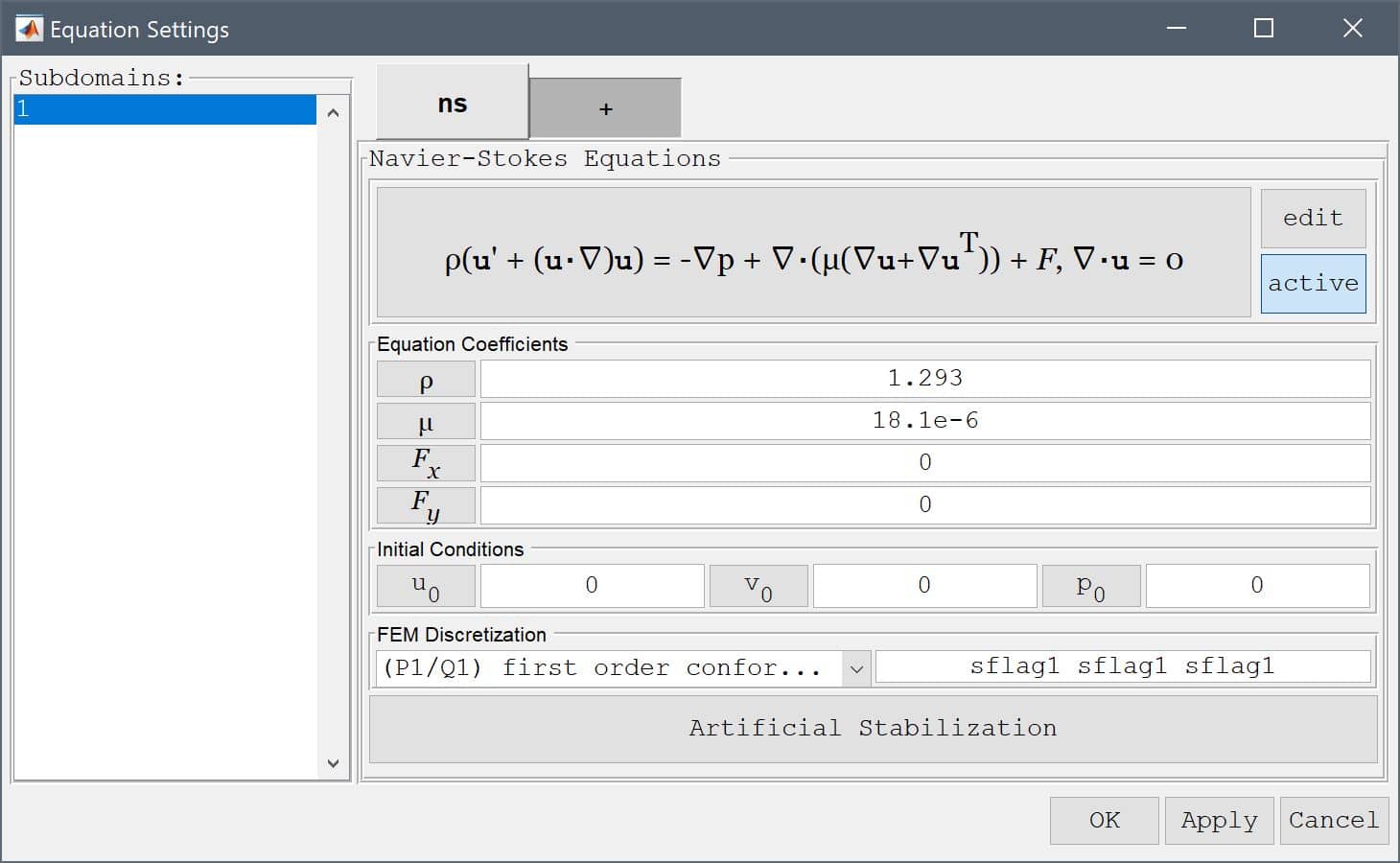
Switch to Equation mode by clicking on the corresponding Mode Toolbar button.
Since the fluid is air, set the density ρ to 1.293 kg/m3 and viscosity µ to 18.1e-6 kg/m/s, in the corresponding edit fields of the Equation Settings dialog box Press OK to finish and close the dialog box.
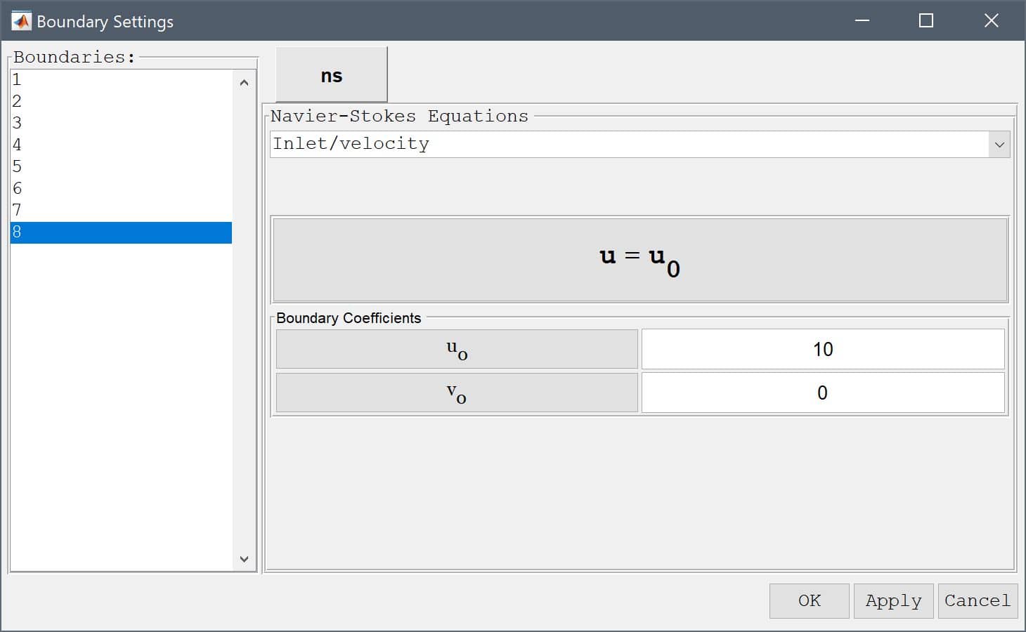
Then select the leftmost boundary (number 8) in the Boundaries list box, and choose the Inlet/velocity boundary condition from the drop-down menu. Enter 10 m/s in the edit field for the x-velocity coefficient u0.
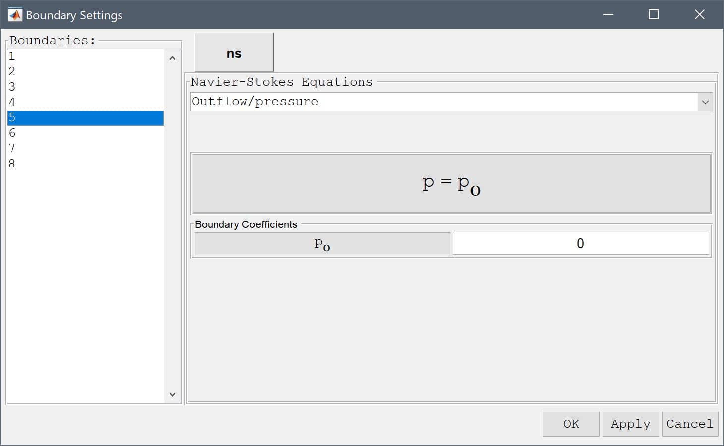
Finally select the right outflow boundary (number 5), and select the Outflow/pressure boundary condition from the drop-down menu. Finish the boundary condition specification by clicking the OK button.
Instead of using the built-in multiphysics solver, the external and dedicated CFD solver OpenFOAM will be used to solve this flow problem. (See the corresponding OpenFOAM solver section in the User's Guide on how to install OpenFOAM.)
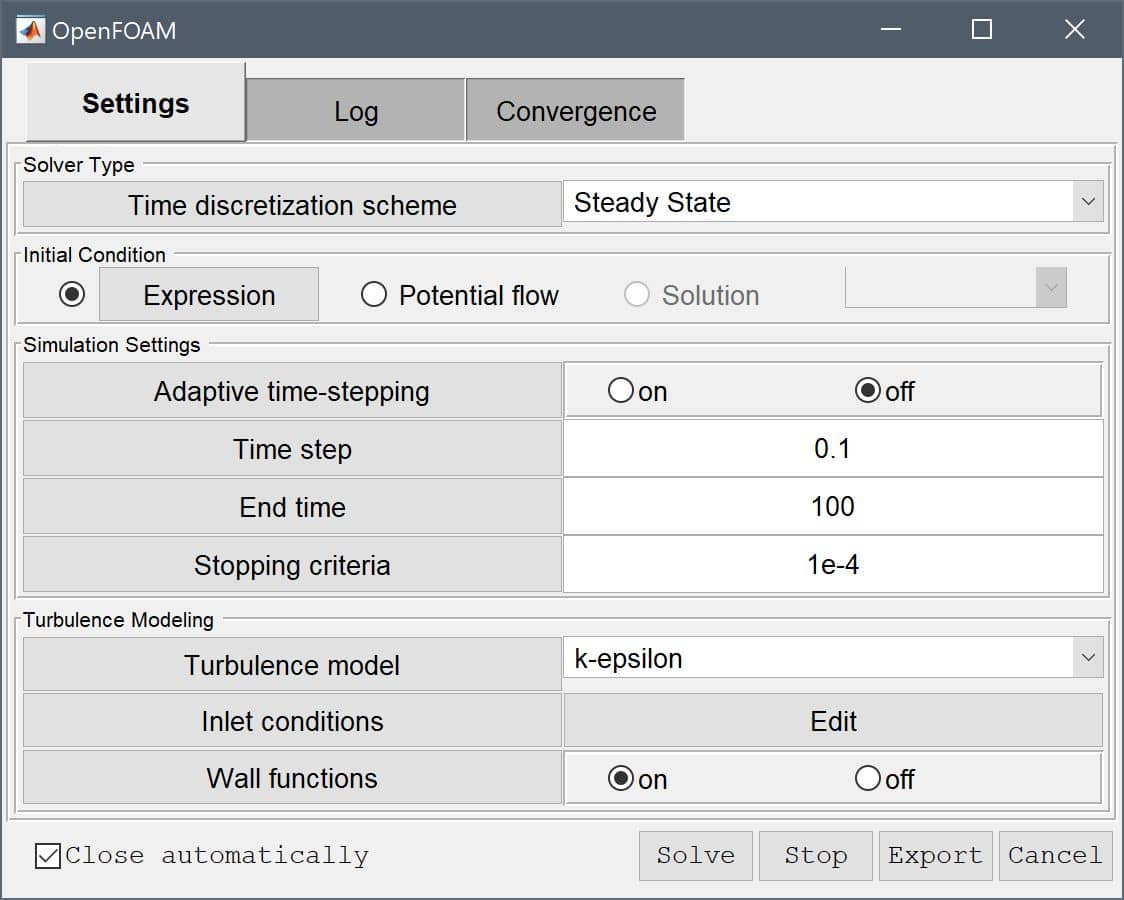
Press the OpenFOAM Toolbar button to open the OpenFOAM solver settings and control panel dialog box. and set the Stopping criteria/tolerance for initial residuals to 1e-4.
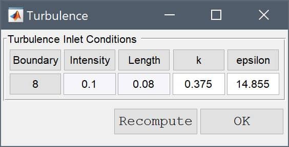
The k and epsilon inlet values can either be estimated from a given turbulence intensity and length scale, or as is done here prescribed directly if the quantities are known.
Enter 0.375 into the edit field for the Turbulent kinetic energy, 14.855 into the edit field for the Turbulent dissipation rate, and press OK.
Advanced users can also use the Edit functionality, to view, fine tune, and modify OpenFOAM dictionaries, as well as export case files for running OpenFOAM simulations separately.
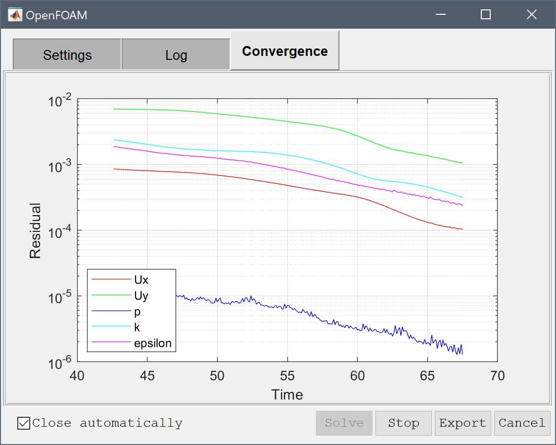
During the solution process one can switch between the convergence tab and the solver output log. The solver will stop when the residuals for all of the flow variables are below the stopping criteria (here 1e-4), or the maximum number of iterations has been reached.
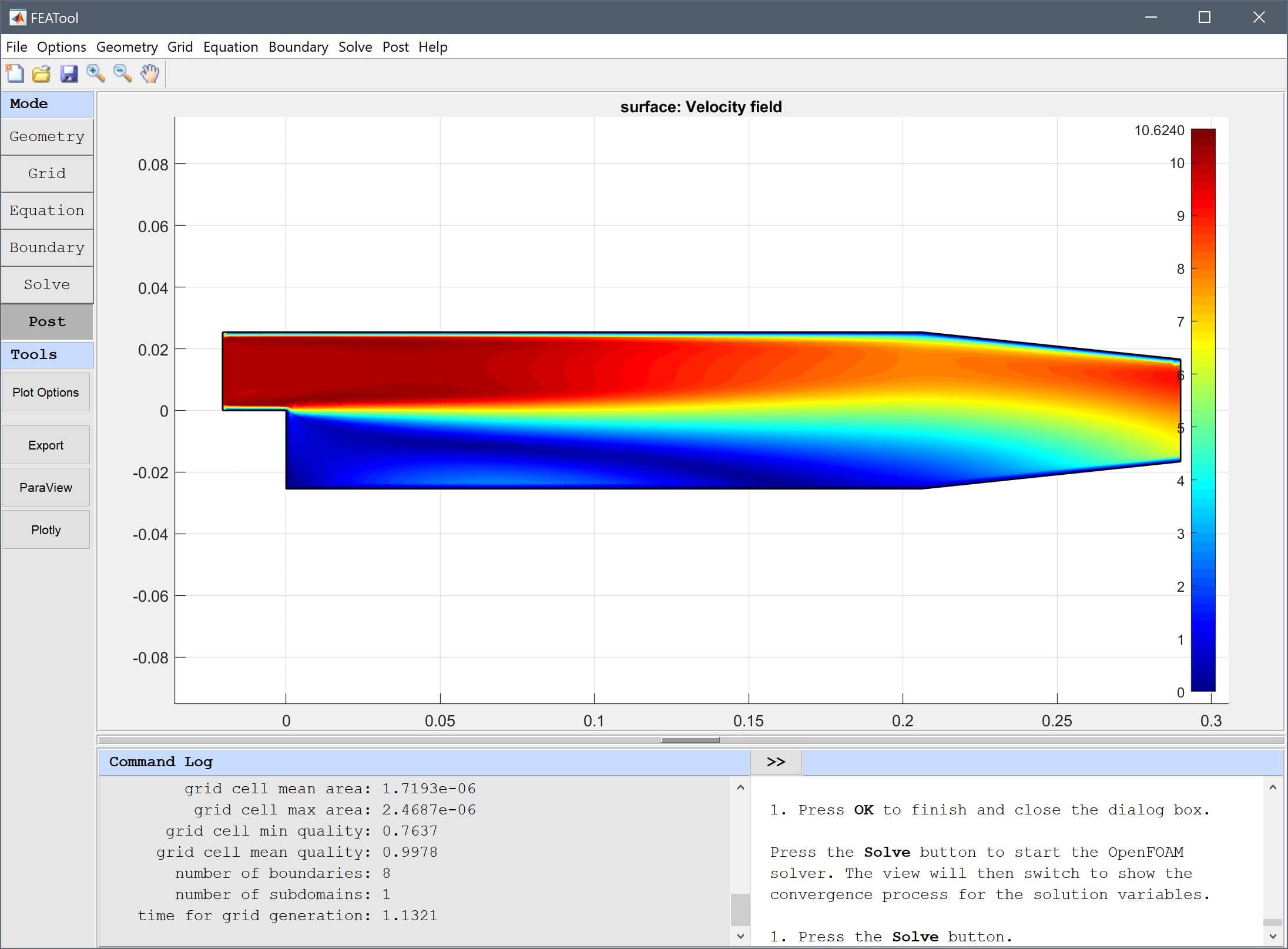
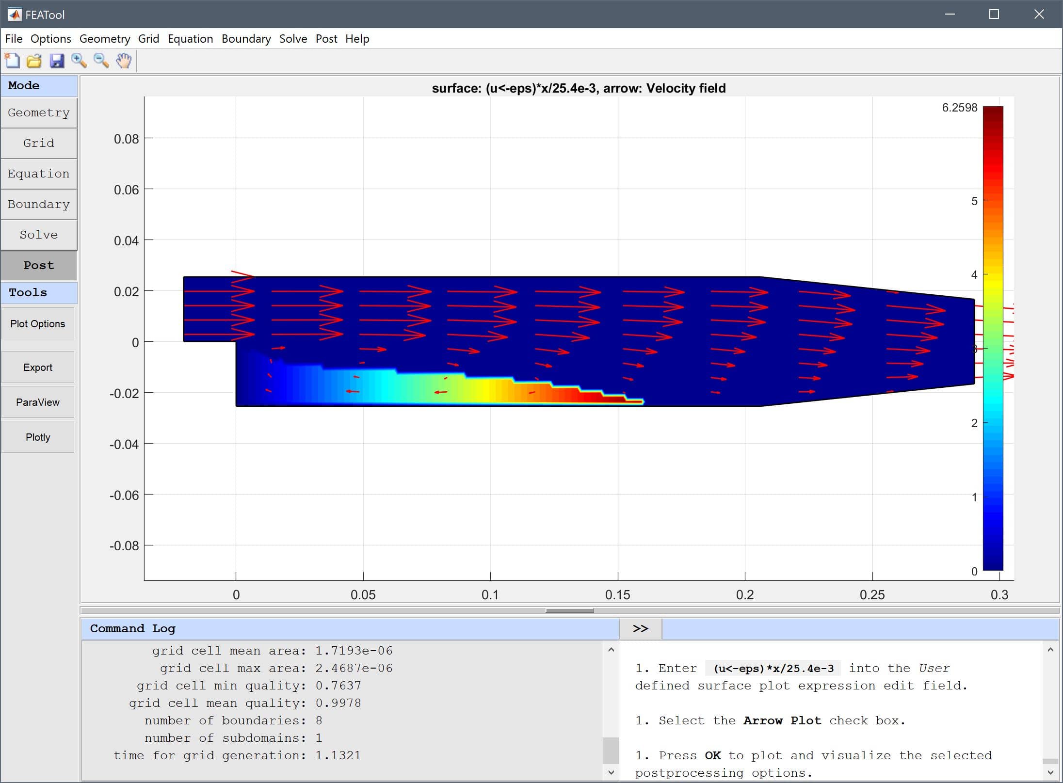
After the solver has finished, the toolbox will automatically switch to postprocessing mode, and show the resulting velocity field. One can see that a recirculation zone has formed after the step.
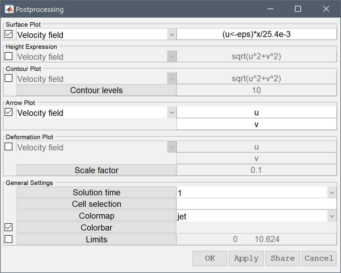
(u<0)*x/25.4e-3 into the Surface Plot expression edit field. The Arrow Plot option can also be turned on to help visualize the flow field.Note that logical or switch type expressions such as a<b evaluate to either 0 or 1, and are here used to limit the plot to the lower half region for which the u velocity is negative.
The resulting plot shows a recirculation zone length of about 6.25 normalized length units, which is quite close to the reference length of 6.4.
The turbulent flow over a backwards facing step fluid dynamics model has now been completed and can be saved as a binary (.fea) model file, or exported as a programmable MATLAB m-script text file, or GUI script (.fes) file.
To visualize the full 3D solution from the planar model, the data can be exported and processed on the MATLAB command line interface (CLI) console with the Export Model Data Struct to MATLAB option from the File menu. The postextrude and postplot functions can then be applied to extrude and visualize the data, for example
fea_extruded = postextrude( fea, 5, 50e-3 );

postplot( fea_extruded, 'surfexpr', 'sqrt(u^2+v^2)', ...
          'parent', figure, 'axis', 'off', 'colorbar', 'off' )
view(25, 25)
[1] Pitz RW, Daily JW. Combustion in a Turbulent Mixing Layer Formed at a Rearward Facing Step. AIAA Journal 21, 1983.