|
|
FEATool Multiphysics
v1.18.1
Finite Element Analysis Toolbox
|
|
|
FEATool Multiphysics
v1.18.1
Finite Element Analysis Toolbox
|
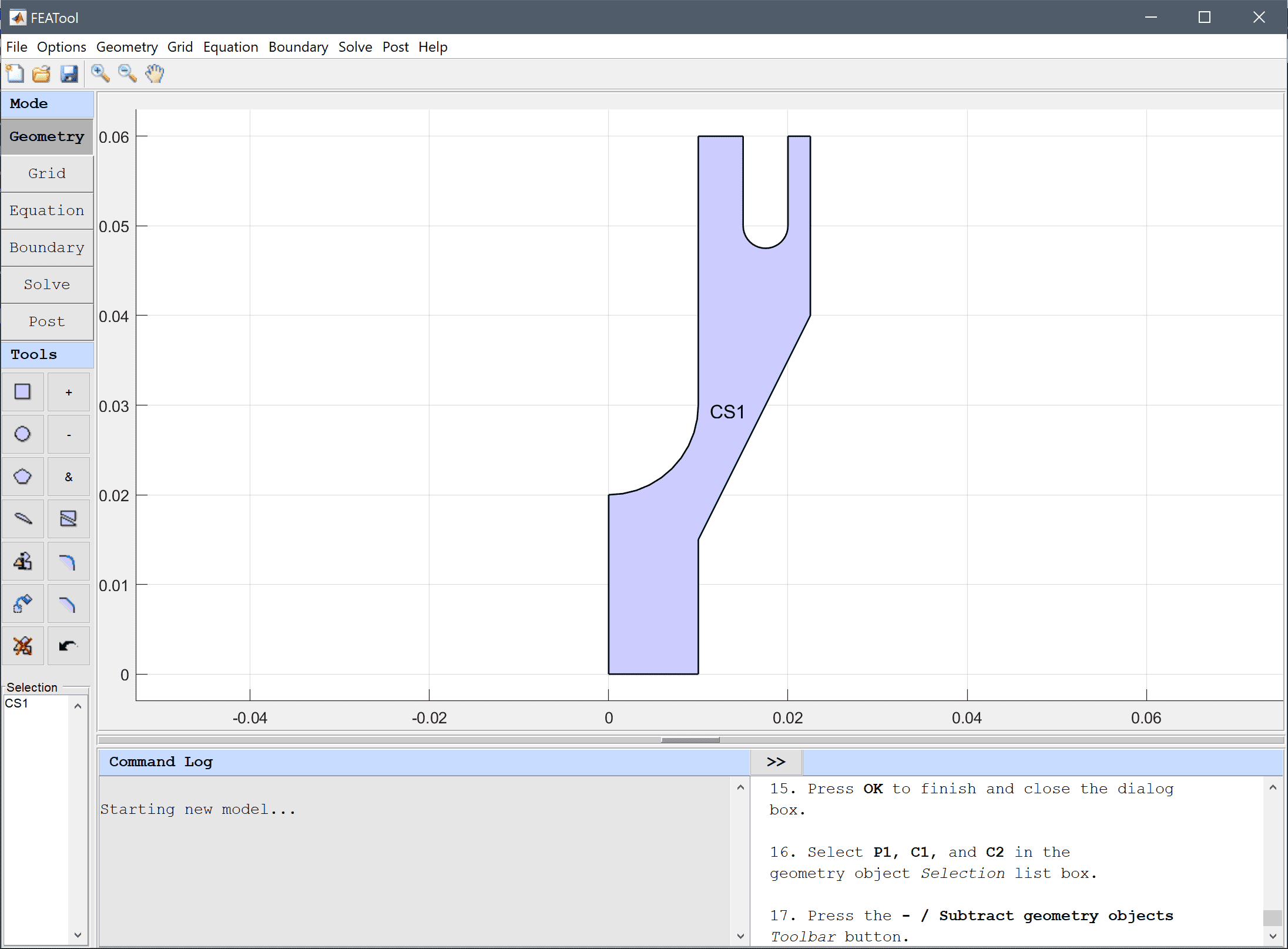
This example models flow of a polymer through an extrusion die with two outlets. This type of flow can for example be found in manufacturing processes of plastic parts. The polymer is assumed to be non-Newtonian, and can be modeled with a shear thinning Bird-Carreau viscosity model. The die is also assumed to be rotationally symmetric, allowing a reduction of the model geometry to an axisymmetric cross section.
This model is available as an automated tutorial by selecting Model Examples and Tutorials... > Fluid Dynamics > Non-Newtonian Flow in an Extrusion Die from the File menu, viewed as a video tutorial, or alternatively, follow the step-by-step instructions below.
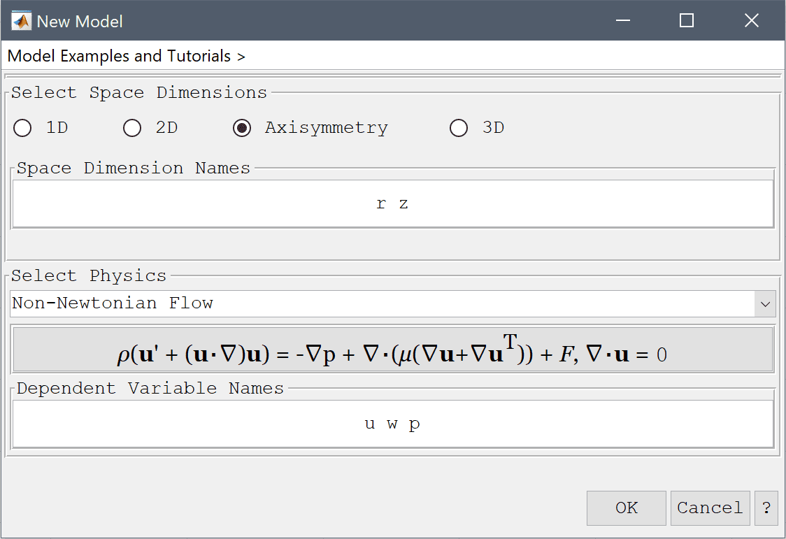
Select the Non-Newtonian Flow physics mode from the Select Physics drop-down menu.
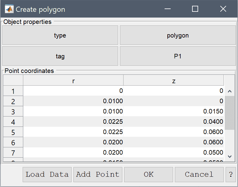
Enter the following data into the Point coordinates table.
| r | z | |
|---|---|---|
| 1 | 0 | 0 |
| 2 | 0.01 | 0 |
| 3 | 0.01 | 0.015 |
| 4 | 0.0225 | 0.04 |
| 5 | 0.0225 | 0.06 |
| 6 | 0.02 | 0.06 |
| 7 | 0.02 | 0.05 |
| 8 | 0.015 | 0.05 |
| 9 | 0.015 | 0.06 |
| 10 | 0.01 | 0.06 |
| 11 | 0.01 | 0.03 |
| 12 | 0 | 0.02 |
0 0.03 into the center edit field.0.01 into the radius edit field.0.0175 0.05 into the center edit field.0.0025 into the radius edit field.Select P1, C1, and C2 in the geometry object Selection list box.
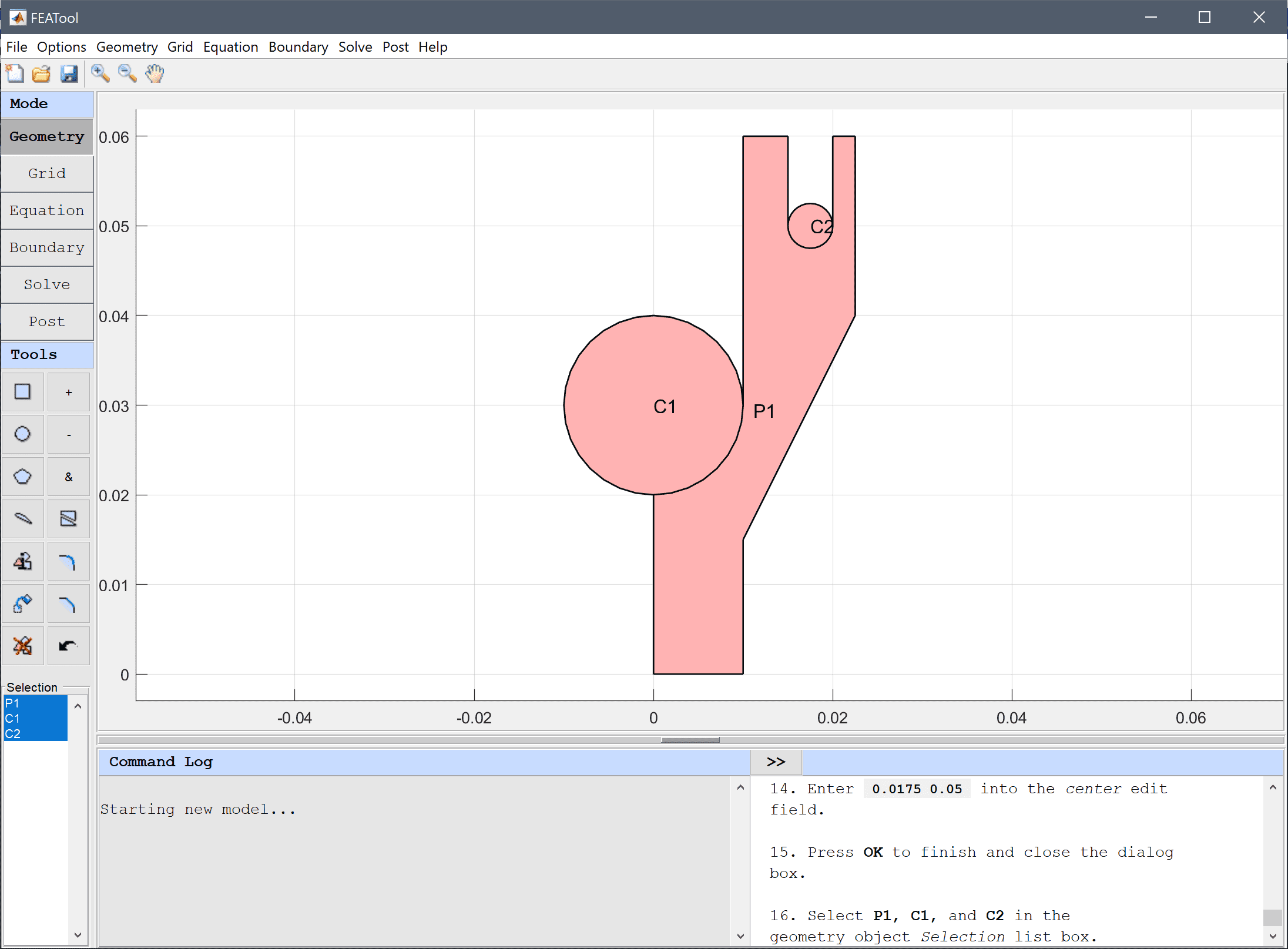
Press the - / Subtract geometry objects Toolbar button.
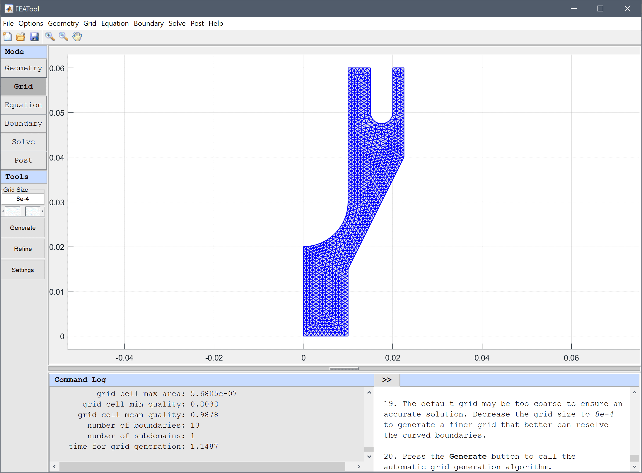
Press the Generate button to call the automatic grid generation algorithm.
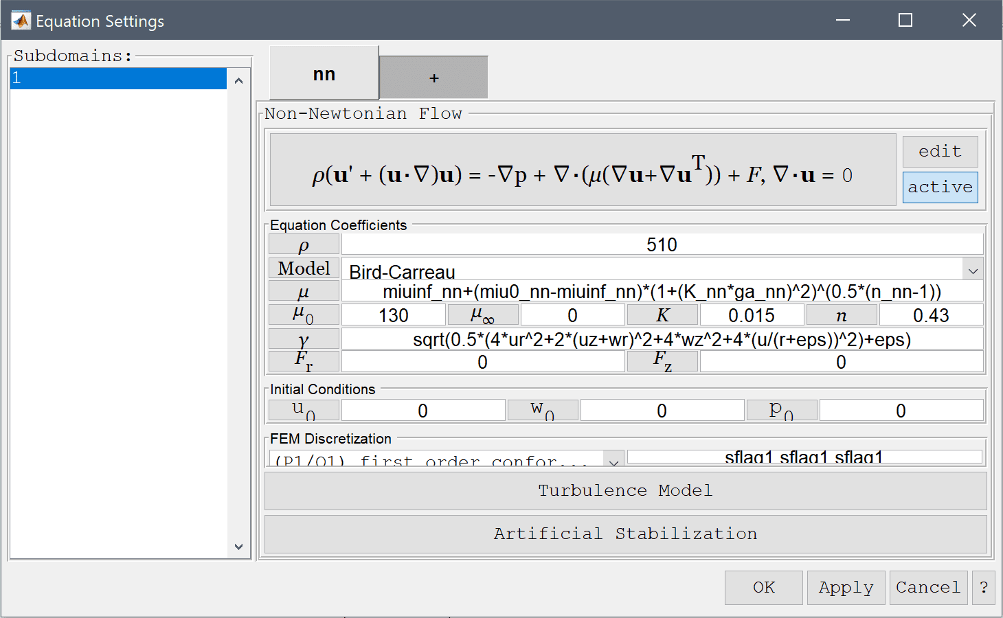
Equation and material coefficients can be specified in Equation/Subdomain mode.
Note that FEATool works with any unit system, and it is up to the user to use consistent units for geometry dimensions, material, equation, and boundary coefficients.
510 into the Density edit field.The Bird-Carreau viscosity model is used here, with a zero shear rate viscosity of 130 Pa s, relaxation time of K = 0.015 1/s, and power index n = 0.43 (indicating a shear thinning pseudo plastic flow regime).
Note that the expression in the edit field for the viscosity now has been updated with the chosen viscosity model.
130 into the Reference viscosity edit field.0 into the Viscosity at infinite shear rate edit field.0.015 into the Model parameter edit field.Enter 0.43 into the Power law index edit field.
A differential pressure of 2e4 Pa is applied between the inlet and the two outlets.
Enter 2e4 into the Pressure edit field.
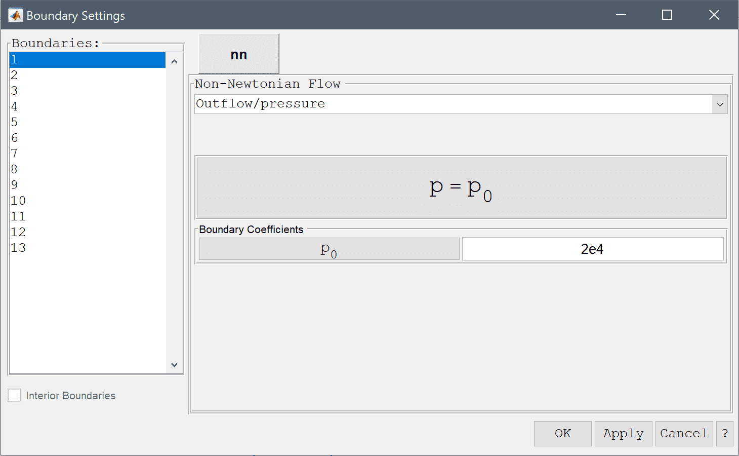
Boundaries along the symmetry axis _(r = 0)_ must be set to the Symmetry and slip condition.
After the problem has been solved FEATool will automatically switch to postprocessing mode, and display the computed velocity field. To change the plot, open the postprocessing settings dialog box by clicking on the Plot Options Toolbar button.
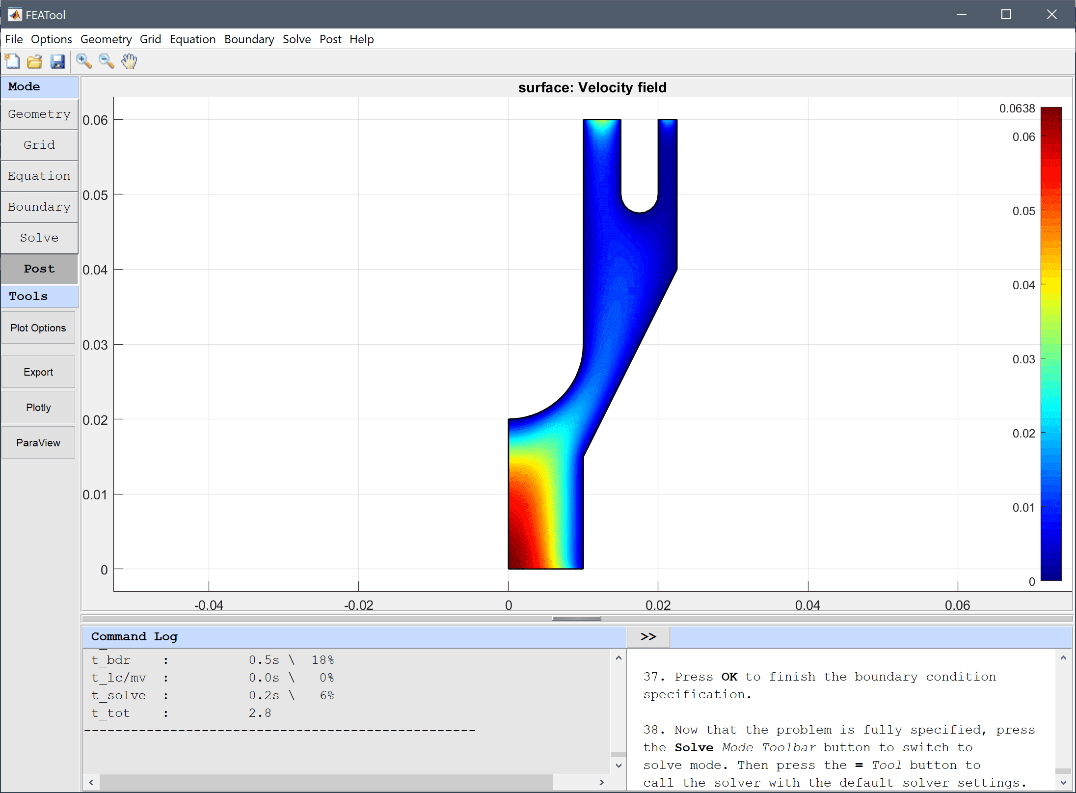
Visualize the effective viscosity and the flow field as arrows.
20 into the Arrow spacing in the r-direction edit field.50 into the Arrow spacing in the z-direction edit field.Select white from the Select arrow color drop-down menu.
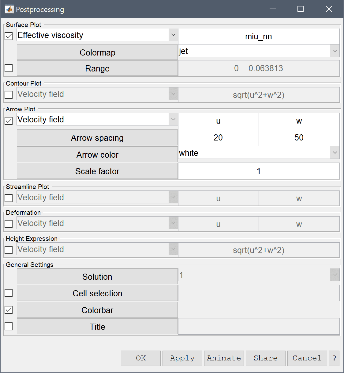
The effective viscosity is decreased in regions where the velocity field exhibit gradients as is expected for shear thinning fluids.
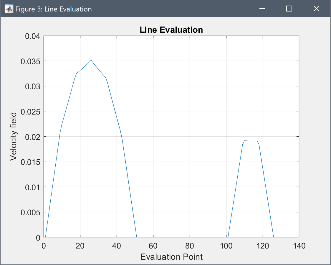
We can also use the line plot functionality to plot and see the difference in the flow field at the outlets.
0.01:1e-4:0.025, in the edit field for Evaluation coordinates in the r-direction.Similarly, enter an expression with a corresponding amount of points at z = 0.06 , 0.06*ones(1,150), in the edit field for Evaluation coordinates in the z-direction.
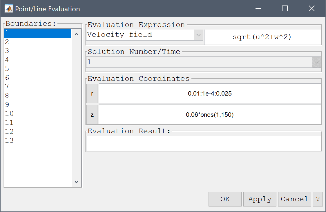
Press OK to plot the curve and close the dialog box.
The non-newtonian flow in an extrusion die fluid dynamics model has now been completed and can be saved as a binary (.fea) model file, or exported as a programmable MATLAB m-script text file, or GUI script (.fes) file.
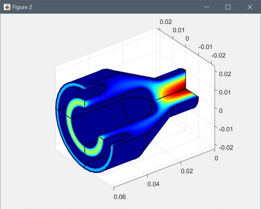
To visualize the full 3D solution the model data can be exported to the MATLAB command line interface (CLI) console with the Export Model Data Struct to MATLAB option from the File menu. The postrevolve and postplot functions can then be applied to revolve and visualize the data, for example
fea_revolved = postrevolve( fea, 24, 0.75 );

postplot( fea_revolved, 'surfexpr', 'sqrt(u^2+w^2)', ...
          'parent', figure, 'axis', 'off', 'colorbar', 'off' )
view(3)
camorbit( 90, 0, 'data', 'y' )