This example illustrates the multiphysics capabilities of FEATool with a simple heat exchanger model featuring both free and forced convection. The model consists of a series of heated pipes around which there is a lower temperature fluid flowing. Two kinds of physics are considered, fluid flow which is modeled by the Navier-Stokes equations and heat transport modeled by a convection and conduction equation for the temperature field. The Boussinesq approximation models the temperature effects on the fluid, and the flow field is coupled to and transports the temperature field. In this way the system is fully two way coupled, the fluid to the temperature and temperature to the fluid.

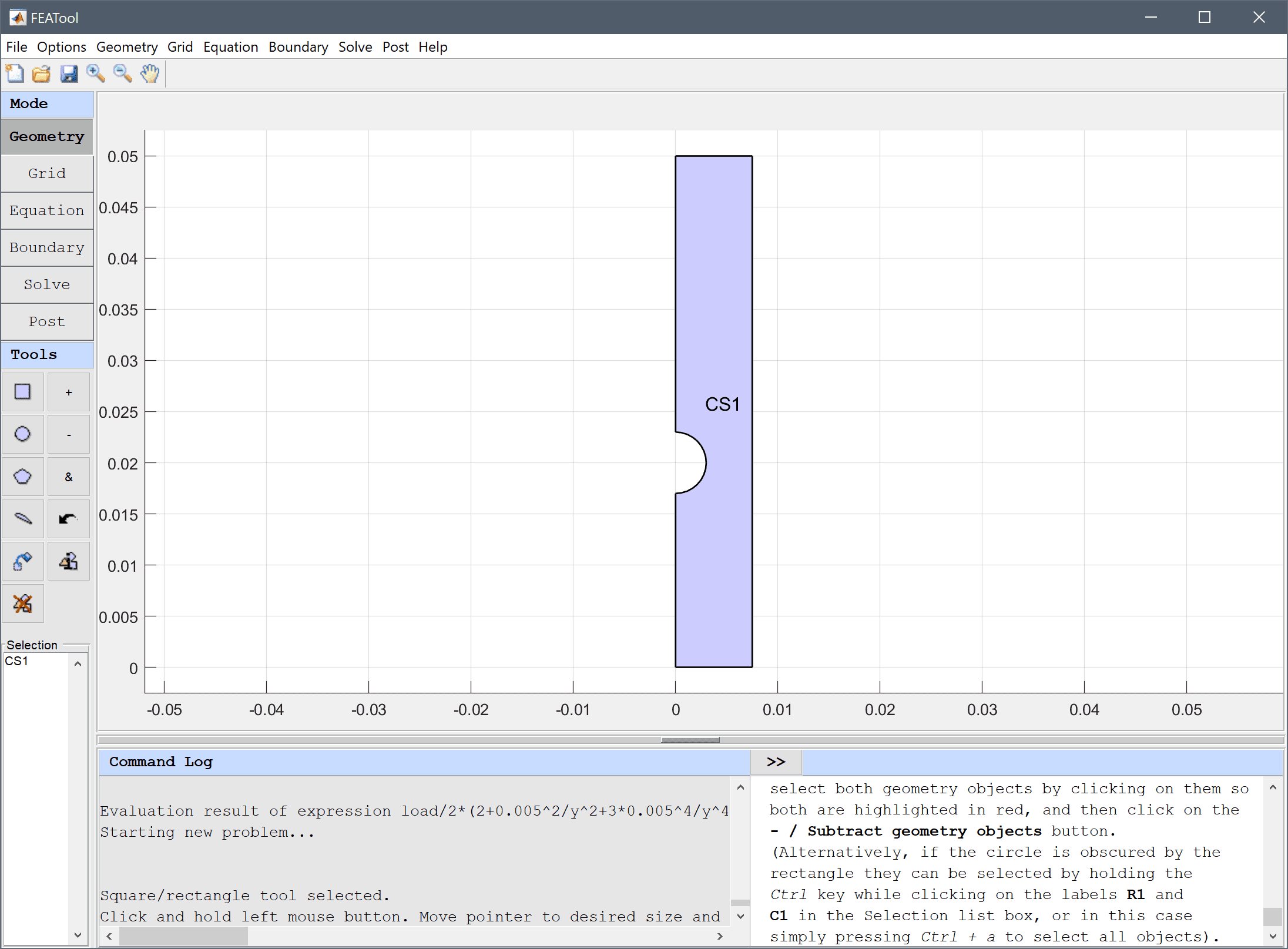
Due to symmetry one can simplify the full geometry and only study a two dimensional slice between the heated pipes. The geometry will therefore consist of a 0.0075 by 0.05 m rectangle from which a half circle with radius 0.003 m centered at (0, 0.02) is removed. The mechanism for heating the pipes is not taken in consideration and are thus assumed to be at a fixed temperature of T_h = 330 K. A cooling fluid flows from the bottom to the top and has an inlet temperature of T_c = 300 K. The other fluid and material parameters can be found in the model tutorial.

Tutorial

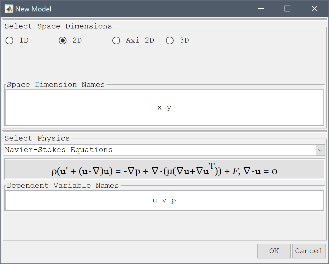
How to set up and solve the heat exchanger example with the FEATool graphical user interface (GUI) is described in the following. Alternatively, this tutorial example can also be automatically run by selecting it from the File > Model Examples and Tutorials > Quickstart menu, or viewed as a video tutorial. Note that the CFDTool interface differ slightly from the FEATool Multiphysics instructions described in the following.

Start MATLAB and launch FEATool by clicking on the corresponding icon in the MATLAB Add-Ons toolbar (or type featool on the command line from the installation directory when not using FEATool as an installed toolbox).
To start a new model click the New Model toolbar button, or select New Model... from the File menu.
In the New Model dialog box, select 2D for the Space Dimensions, and select Navier-Stokes Equations from the Select Physics drop-down menu. An additional physics mode will be added later to couple and model heat transfer effects. Leave the space dimension and dependent variable names to their defaults and press OK to finish the physics mode selection. (Note that for CFDTool the physics selection is done in the Equation settings dialog box.)

The geometry of the heat exchanger cross section can be created by first making a square and a circle, and then subtracting the circle from the square.

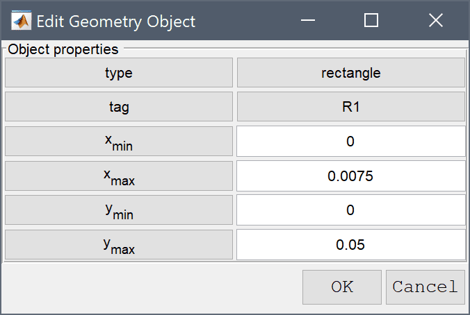
To create a rectangle, first click on the Create square/rectangle Toolbar button. Then left click in the main plot axes window, and hold down the mouse button. Move the mouse pointer to draw the shape outline, and release the button to finalize the shape.
The geometry object properties must now be edited to set the correct size and position of the rectangle. To do this, click on the rectangle R1 to select it which highlights it in red. Then click on the Inspect/edit selected geometry object Toolbar button, and change the min and max coordinates of the rectangle so they span between 0 and 0.0075 in the x-direction, and 0 and 0.05 in the y-direction.
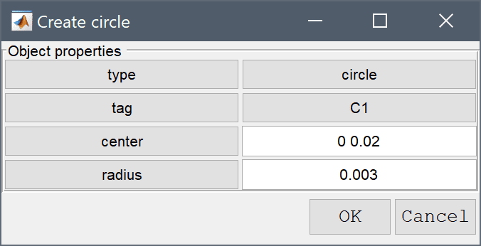
Select Circle from the Geometry menu.
Define a circle with center at (0, 0.02), and radius equal to 0.003. Press OK to close the dialog box and generate the circle.
To subtract the circle from the rectangle first select both geometry objects by clicking on them so both are highlighted in red, and then click on the - / Subtract geometry objects button. (Alternatively, if the circle is obscured by the rectangle they can be selected by holding the Ctrl key while clicking on the labels R1 and C1 in the Selection list box, or in this case simply pressing Ctrl + A to select all objects).
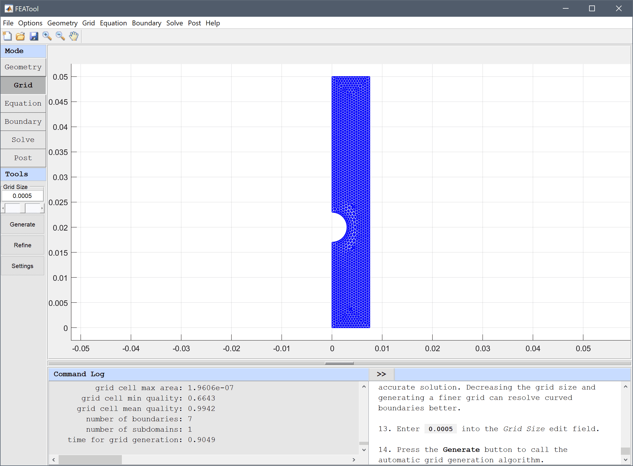
Switch to Grid mode by clicking on the corresponding Mode Toolbar button.

The default grid may be too coarse to ensure an accurate solution. Decreasing the grid size and generating a finer grid can resolve curved boundaries better.

Enter 0.0005 into the Grid Size edit field, and press the Generate button to call the automatic grid generation algorithm.
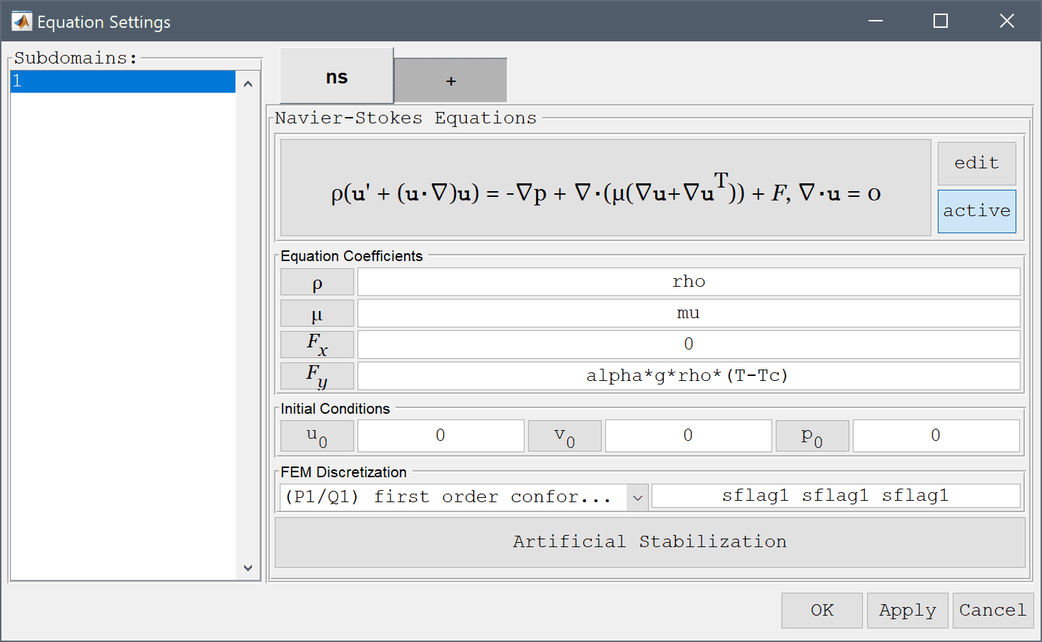
Switch to Equation mode by clicking on the corresponding Mode Toolbar button.
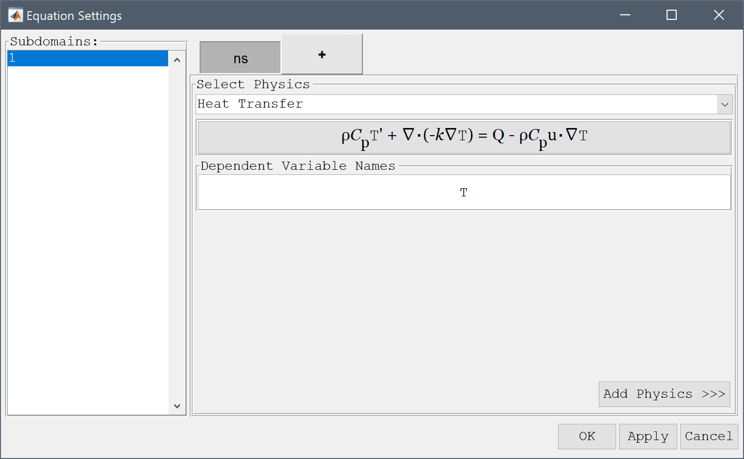
Equation and material coefficients are specified in Equation/Subdomain mode. In the Equation Settings dialog box enter the following coefficients, rho for the density, ρ, mu for the viscosity, µ, and alpha*g*rho*(T-Tc) for the volume force in the y-direction, F_y. (Note that the Equation Settings dialog box may look different for CFDTool.)
A heat transfer physics must also be added. To access the multiphysics selection and add another physics mode press the plus + tab and select Heat Transfer from the Select Physics drop-down menu. Add the selection by pressing the Add Physics >>> button.

Note that each physics mode will have its own tab for Subdomain and Equation settings, and Boundary conditions. Moreover, FEATool works with any unit system, and it is up to the user to use consistent units for geometry dimensions, material, equation, and boundary coefficients.

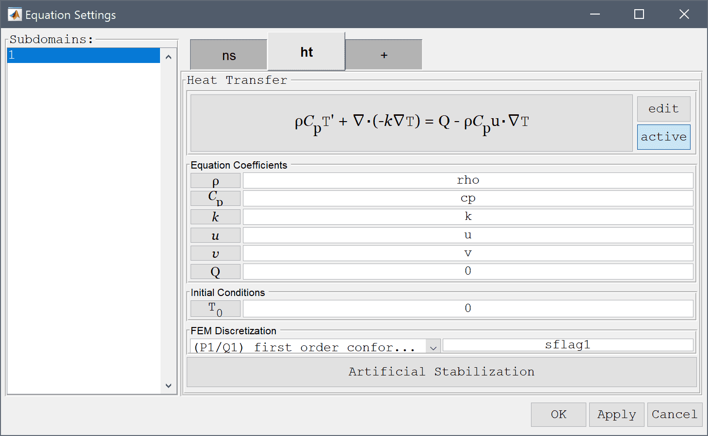
In the ht Equation Settings tab, set the density to rho, heat capacity to cp, and thermal conductivity to k, respectively. The convective velocities should be coupled from the Navier-Stokes equations physics mode, to do this enter u and v in the corresponding edit fields (as these are the default names of the dependent variables for the velocities). Press OK to finish with the equation coefficient specifications.

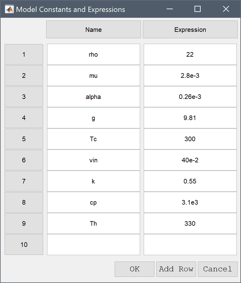
The Model Constants and Expressions functionality can be used to define and store convenient expressions which then are available in the point, equation, boundary coefficients, and as postprocessing expressions. Here it is used to define the material and fluid parameters.

Press the Constants Toolbar button, or select the corresponding entry from the Equation menu, and enter the following variables in the Model Constants and Expressions dialog box. Press Enter after the last expression or use the Add Row button to expand the expression list.

Name	Expression
rho	22
mu	2.8e-3
alpha	0.26e-3
g	9.81
Tc	300
vin	40e-2
k	0.55
cp	3.1e3
Th	330

Switch to Boundary mode by clicking on the corresponding Mode Toolbar button.

Boundary conditions are defined in Boundary Mode and describes how the model interacts with the external environment.

First select the ns tab, which allows for specifying boundary conditions for the Navier-Stokes equations physics mode. Then select all vertical boundaries (here 2, 4, and 7), and choose Symmetry/slip from the drop down box. Switch to the heat transfer physics mode by selecting the ht tab and choose the Thermal insulation/symmetry boundary condition.

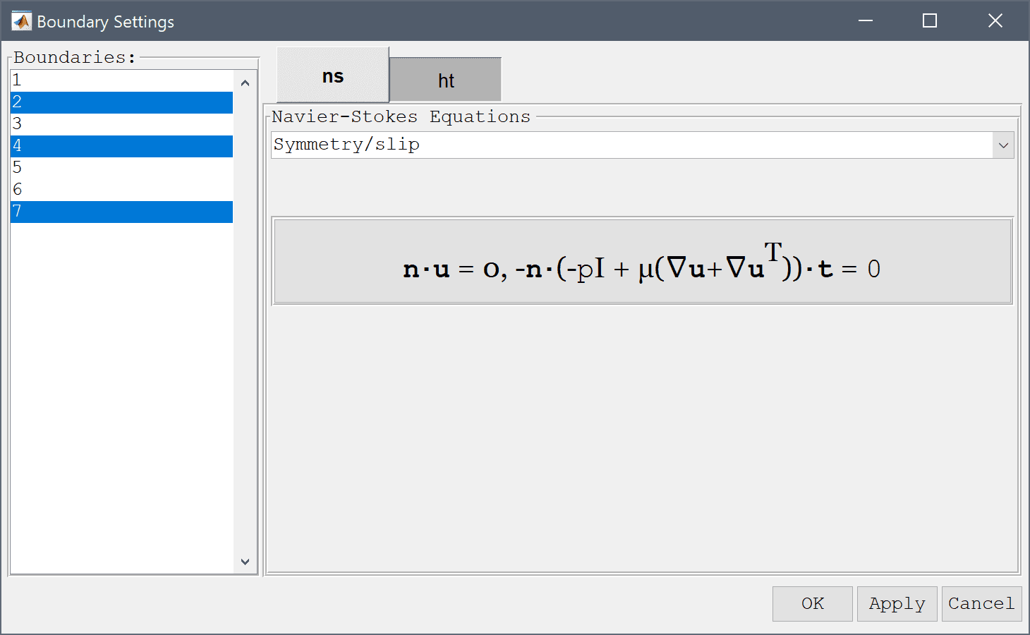
The selected boundaries will be highlighted in red.

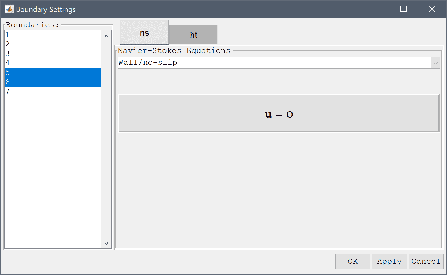
Continue with the top boundary (number 3) which is the outflow. Select Outflow/pressure for the Navier-Stokes physics mode and Convective flux/outflow for the heat transfer mode.
The bottom boundary (number 1) is the inflow and should be prescribed with the constant velocity vin in the y-direction by using the Inlet/velocity condition. The Temperature should here be fixed to the low temperature Tc
Lastly, the boundaries on the cylinder (5 and 6) are walls and should be prescribed with Wall/no-slip boundary conditions for the velocity. For the Temperature the constant high temperature Th should be prescribed.
Now that the problem is fully specified, press the Solve Mode Toolbar button to switch to solve mode. Then press the = Tool button to call the solver with the default solver settings.

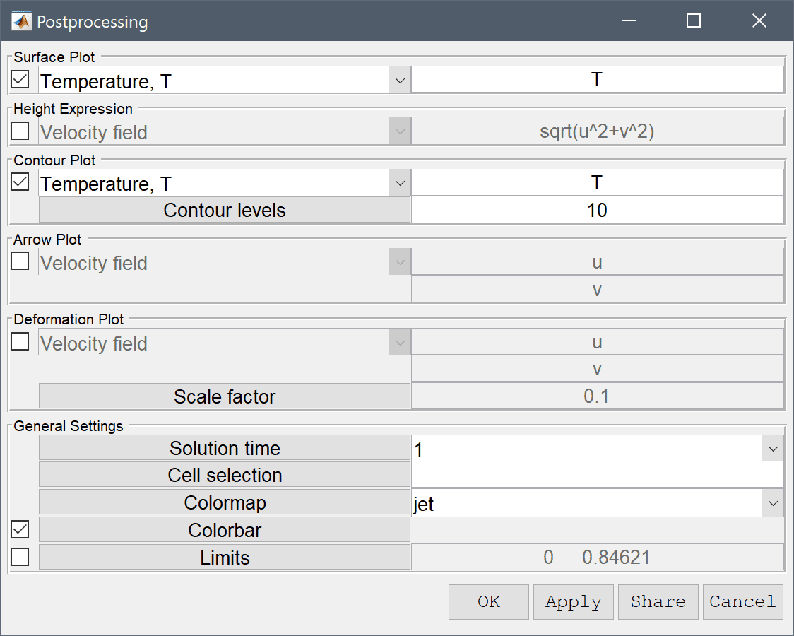
From the resulting flow field one can see that fluid is accelerated when it passes between the cylinders. To visualize the temperature field, open the Plot Options and postprocessing settings dialog box and select to plot and visualize the Temperature, T as both surface and contour plots.

The temperature plot show that the fluid is heated around the hot cylinder and follows the flow upwards.

FEATool also allows for advanced postprocessing such as boundary integration. Integrate the expression (T-Tc)/w over the outflow boundary (where w = 0.0075 is the width of the domain) to find the change in the mean temperature.

Select Boundary Integration... from the Post menu.
Select 3 in the Boundaries list box.
Enter (T-Tc)/0.0075 into the Integration Expression edit field.
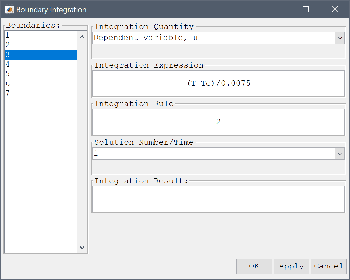
Press OK or Apply to calculate and show the result of the boundary integration.

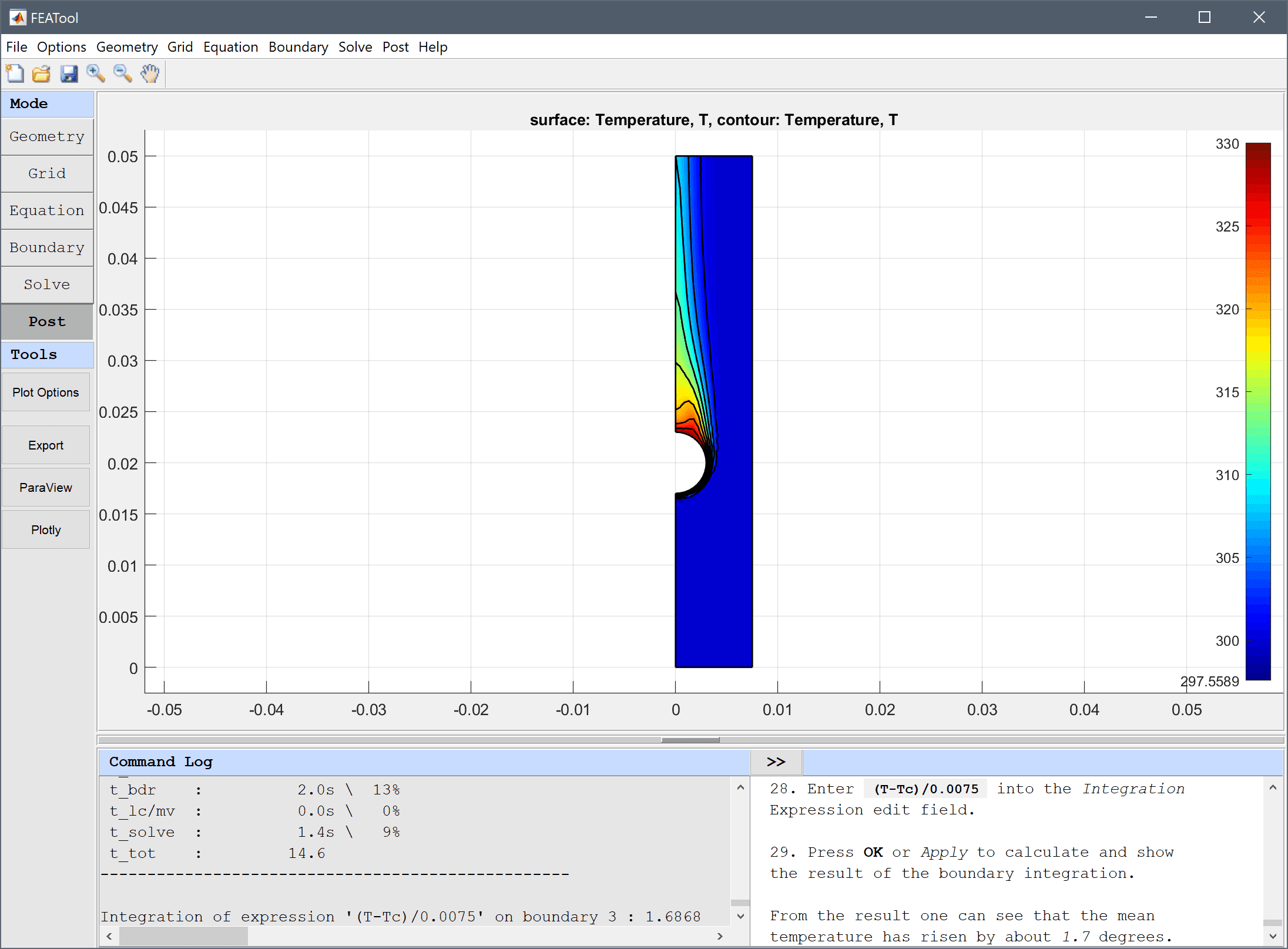
From the result one can see that the mean temperature along the outflow boundary has risen by about 1.7 degrees.

The heat exchanger multiphysics model has now been completed and can be saved as a binary (.fea) model file, or exported as a programmable MATLAB m-script text file (available as the example ex_heat_exchanger1 script file), or GUI script (.fes) file.

CLI Postprocessing

To visualize the full 3D solution the model data can be exported to the MATLAB command line interface (CLI) console with the Export Model Data Struct to MATLAB option from the File menu. The following advanced script can then be used to recreate the full model

fig = figure();

% Create full 3D geometry.
for i=1:5
  offset = (i-1) * 0.015;
  geom.objects{i} = gobj_cylinder( [0+offset 0.02 -0.02], [0.003], [0.04], [0 0 1], sprintf( 'C%d', i ) );
end

% Get surface patch data.
h = postplot( fea, 'surfexpr', 'T', 'colorbar', 'off', 'parent', fig );
hp = findall( h, 'Type', 'patch' );
pdata = get( hp, {'vertices', 'faces', 'facevertexcdata'} );
delete(h)


% Plot surface patches.
xoffset = 0.015;
for i=0:4
  p = pdata{1};
  p(:,1) = p(:,1) + xoffset*i;
  patch( 'vertices', p, 'faces', pdata{2}, 'facevertexcdata', pdata{3}, ...
         'facecolor', 'interp', 'linestyle', 'none' );
end

for i=0:4
  p = pdata{1};
  p(:,1) = -p(:,1) + xoffset*i;
  patch( 'vertices', p, 'faces', pdata{2}, 'facevertexcdata', pdata{3}, ...
         'facecolor', 'interp', 'linestyle', 'none' );
end
alpha(0.5)

% Plot surface, contour, and arrow plots on center column.
fea.grid.p(1,:) = fea.grid.p(1,:) + 2*xoffset;
postplot( fea, 'surfexpr', 'T', 'isoexpr', 'T', ...
          'arrowexpr', {'u','v'}, 'arrowcolor', 'w', ...
          'colorbar', 'off', 'parent', fig );
fea.grid.p(1,:) = -fea.grid.p(1,:) + 5*xoffset;
postplot( fea, 'surfexpr', 'T', 'isoexpr', 'T', ...
          'arrowexpr', {'u','v'}, 'arrowcolor', 'w', ...
          'colorbar', 'off', 'parent', fig );

% Plot geometry.
plotgeom( geom, 'labels', 'off', 'highlight', 1:5, 'parent', fig )

% Camera settings.
axis tight
axis equal
axis off
view(35, 35)
camorbit( -90, 0, 'data', 'x' )

Tutorial

CLI Postprocessing

Video