|
|
FEATool Multiphysics
v1.18.1
Finite Element Analysis Toolbox
|
|
|
FEATool Multiphysics
v1.18.1
Finite Element Analysis Toolbox
|
This example is a well known benchmark test case from structural mechanics, a thin plate with a circular hole in the center is subjected to a load and stretched along the horizontal axis.
The plate is thin enough to satisfy the two dimensional plane stress approximation, and since both the problem and solution will be symmetric around the hole it is enough to model a quarter of the plate. The computational geometry here therefore consist of a 0.05 by 0.05 m square with a quarter of a circle with radius 0.005 m removed from one corner. Due to the symmetry the displacement of the left edge of the plate should be zero in the x-direction, and similarly the y-displacement for the lower edge should also be zero. Furthermore, a horizontal force of 1000 N is applied to the right edge. With a plate thickness of 0.001 m, the resulting load will be 1000/(2·0.05·0.001) N/m2.
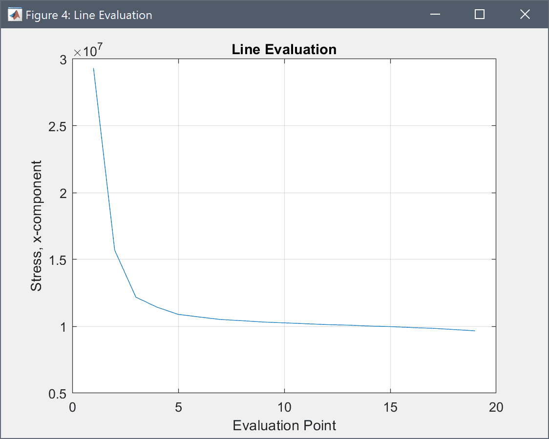
Assuming that the plate is made of steel with a Poisson ratio of 0.3 and modulus of elasticity 210·109 Pa then it is expected that the maximum stress in the x-direction will be three times the stress of a plate without a hole, that is σx = 3·1000/(2·0.05·0.001) = 3·107 Pa [1]. The computed stress along the left side vertical boundary is compared against the theoretical reference results in the figure, clearly showing very good agreement.
How to set up and solve the thin plate with hole example with the FEATool graphical user interface (GUI) is described in the following. Alternatively, this tutorial example can also be automatically run by selecting it from the File > Model Examples and Tutorials > Quickstart menu, or viewed as a video tutorial.
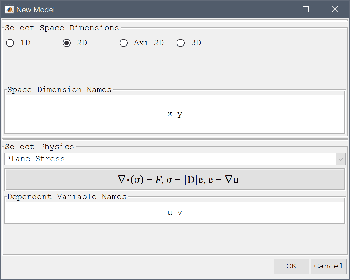
featool on the command line from the installation directory when not using FEATool as an installed toolbox).In the New Model dialog box, select 2D for the Space Dimensions, and then choose Plane Stress from the Select Physics drop-down menu. Leave the space dimension and dependent variable names to their defaults, and press OK to finish the physics mode selection.
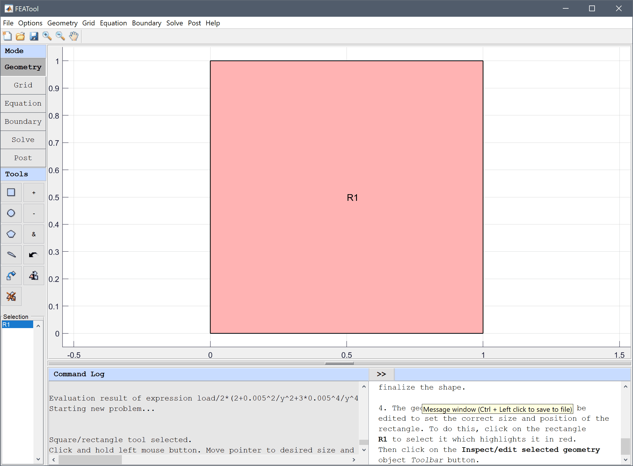
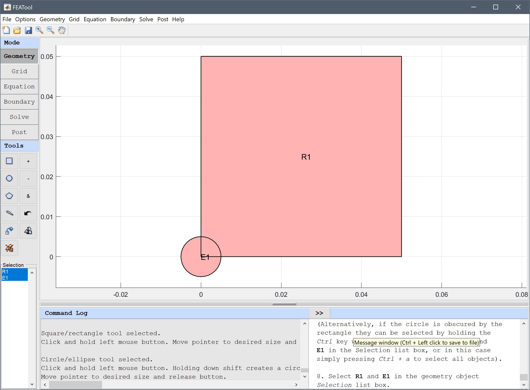
The geometry of the plate can be created by first making a square for the base, and then subtracting a circle from the lower right corner.
To create a rectangle, first click on the Create square/rectangle Toolbar button. Then left click in the main plot axes window, and hold down the mouse button. Move the mouse pointer to draw the shape outline, and release the button to finalize the shape.
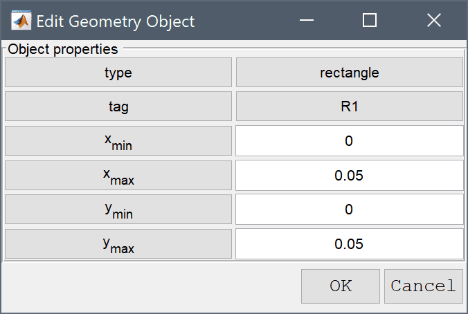
In the Edit Geometry Object dialog box, change the x/ymin and x/ymax point coordinates to define a rectangle with length and height 0.05 and lower left corner at the origin (0, 0). Finish editing the geometry object and close the dialog box by clicking OK.
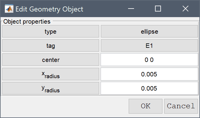
The object properties of the ellipse E1 must be changed to make a circle with radius 0.005 centered at (0, 0). Click on the ellipse E1 to select it and highlights it in red, and use the Inspect/edit selected geometry object tool to set the center and radius.
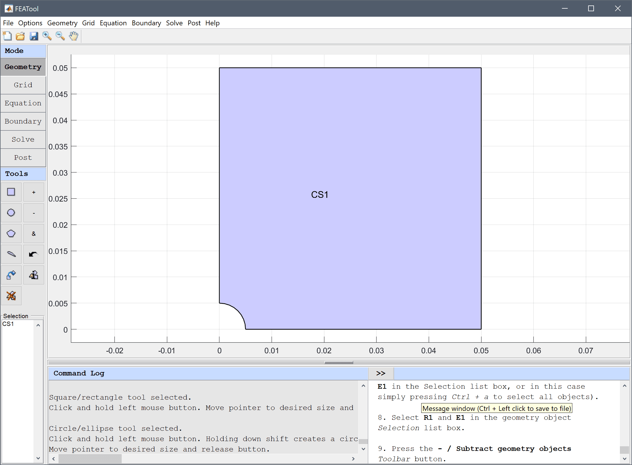
To subtract the circle from the rectangle first select both geometry objects by clicking on them so both are highlighted in red, and then click on the - / Subtract geometry objects button. (Alternatively, if the circle is obscured by the rectangle they can be selected by holding the Ctrl key while clicking on the labels R1 and E1 in the Selection list box, or in this case simply pressing Ctrl + A to select all objects).
Select R1 and E1 in the geometry object Selection list box.
Press the - / Subtract geometry objects Toolbar button.
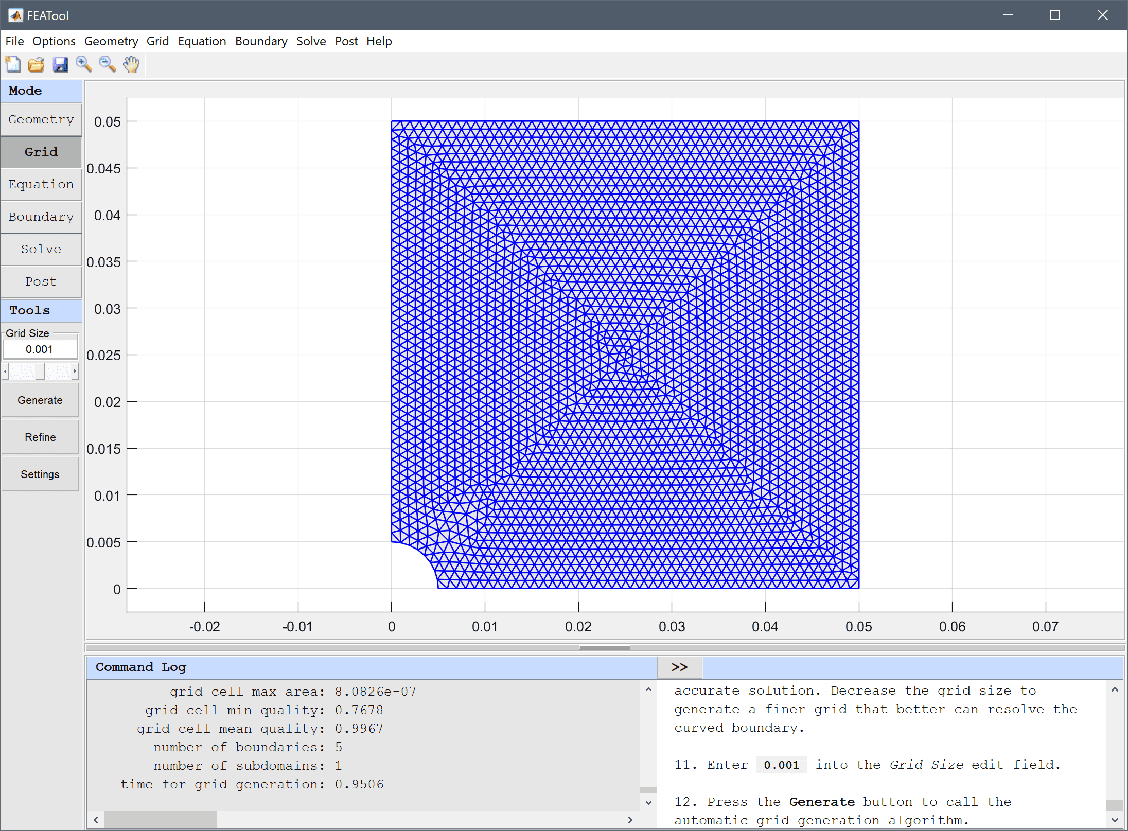
The default grid may be too coarse to ensure an accurate solution. Decrease the grid size to generate a finer grid that better can resolve the curved boundary.
0.001 into the Grid Size edit field.Press the Generate button to call the automatic grid generation algorithm.
Equation and material coefficients can be specified in Equation/Subdomain mode. In the Equation Settings dialog box that automatically opens, enter 0.3 for the Poisson's ratio and 210e9 for the Modulus of elasticity. The other coefficients can be left to their default values. Press OK to finish the equation and subdomain settings specification.
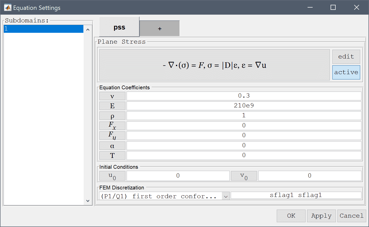
Note that FEATool works with any unit system, and it is up to the user to use consistent units for geometry dimensions, material, equation, and boundary coefficients.
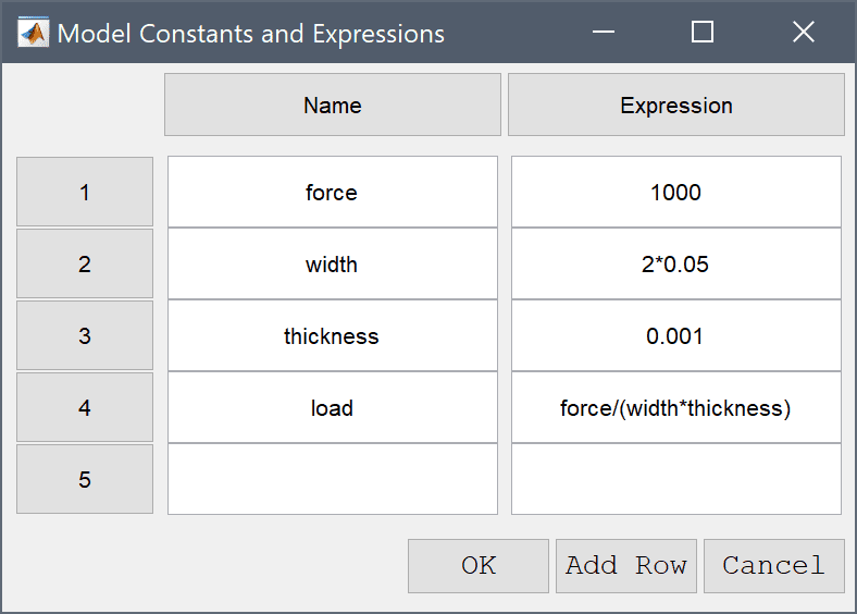
A convenient way to define and store coefficients, variables, and expressions is using the Model Constants and Expressions functionality. The defined expressions can then be used in point, equation, boundary coefficients, as well as postprocessing expressions, and can easily be changed and updated in a single place.
load force, press the Constants Toolbar button, or select the corresponding entry from the Equation menu, and enter the following variables in the Model Constants and Expressions dialog box.| Name | Expression |
|---|---|
| force | 1000 |
| width | 2*0.05 |
| thickness | 0.001 |
| load | force/(width*thickness) |
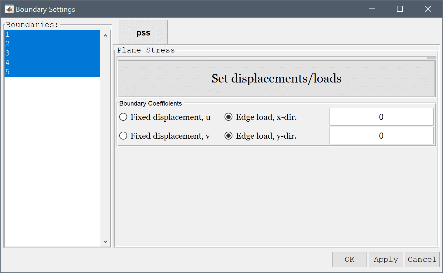
Boundary conditions are defined in Boundary Mode and describes how the model interacts with the external environment.
In the Boundary Settings dialog box, first select all boundaries and set all conditions to Edge loads with a value of zero 0 (The selected boundaries will be shown highlighted in red).
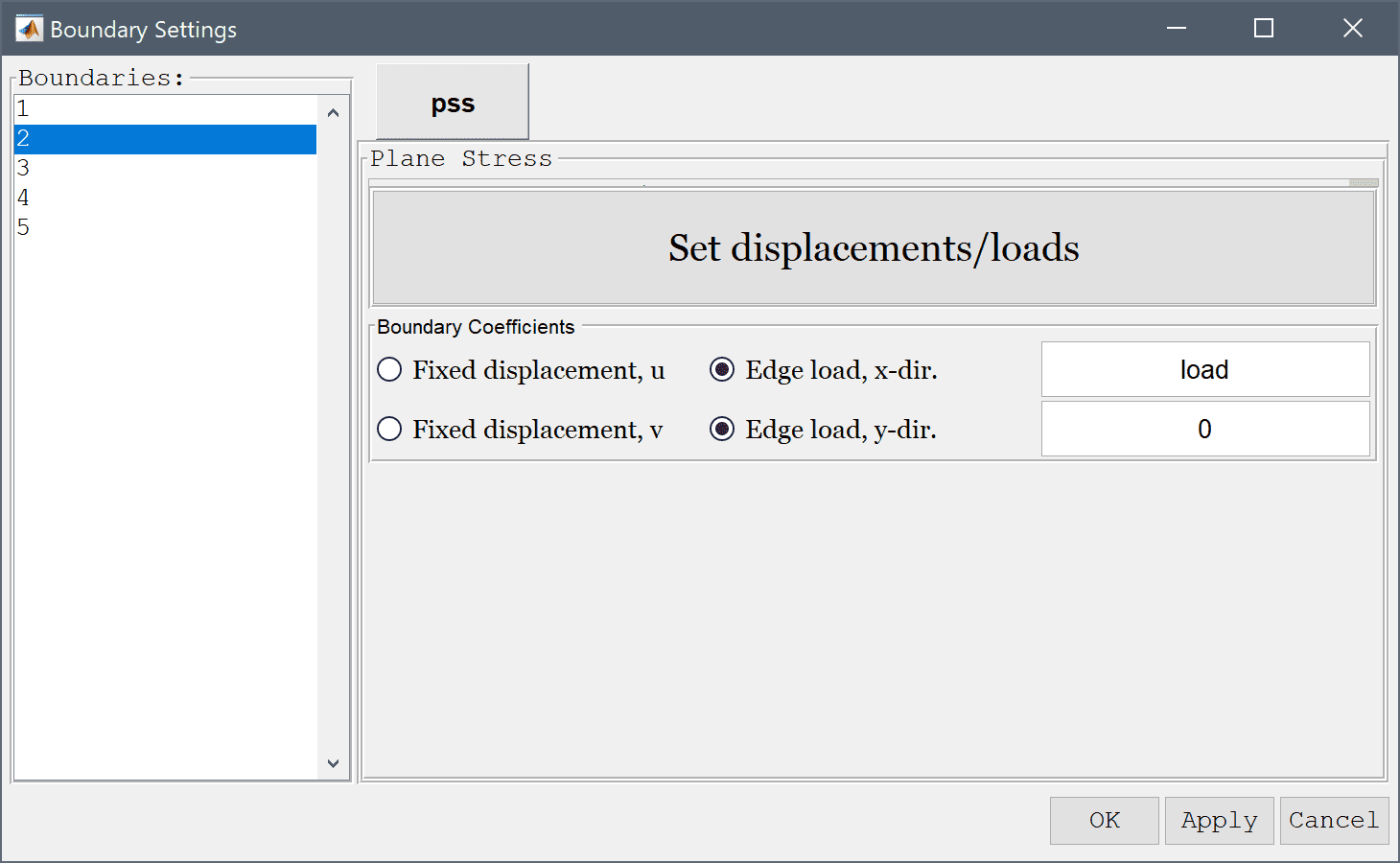
Lastly, select both Edge load boundary conditions for the right boundary (number 3). Set the edge load in the x-direction on this boundary to the previously defined load expression. Finish the boundary condition specification by clicking the OK button.
Select Stress, x-component from the Predefined surface plot expressions drop-down menu.
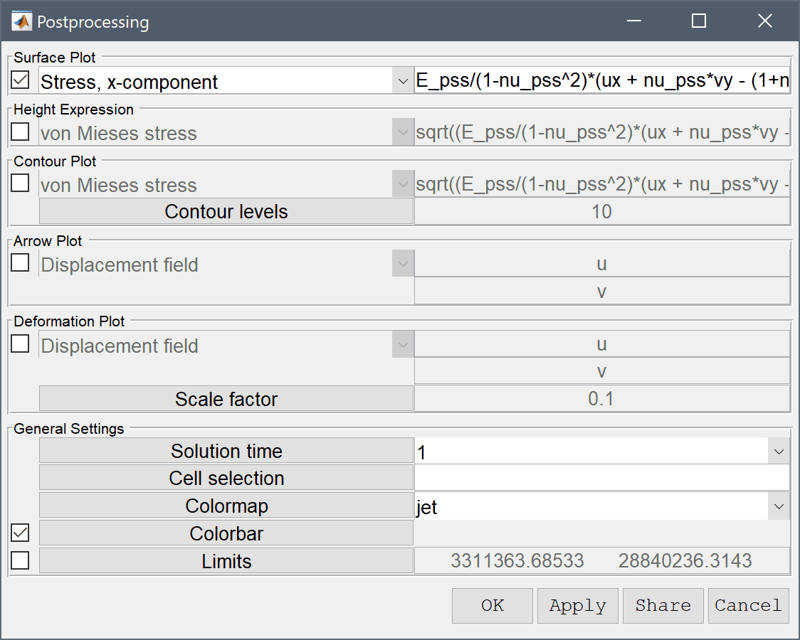
One can evaluate and find the value of a plotted expression by directly clicking on the surface plot. Alternatively, the Min/Max Evaluation postprocessing tool can be used to find the maximum tangential stress.
Press OK or Apply to calculate and show the minima and maxima.
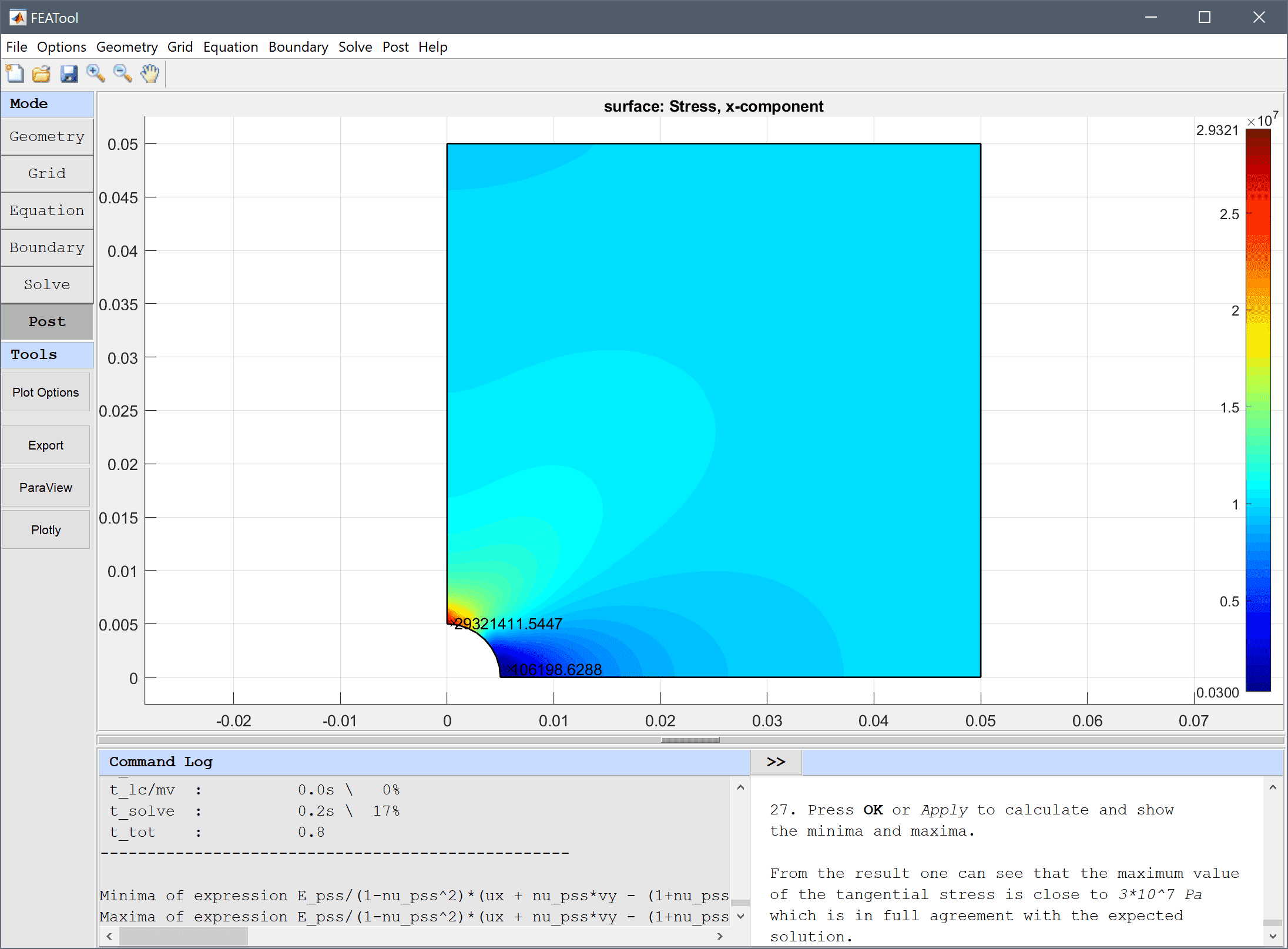
From the result one can see that the maximum value of the tangential stress is close to 3·107 Pa which is in full agreement with the expected solution.
The stress along the left symmetry axis can also be plotted with the Point/Line Evaluation feature and compared with the equivalent of the analytical solution F/A/2*(1+r2/y2+3*r4/y4).
To evaluate and stress on the left boundary, select boundary number 5 in the Boundaries list box.
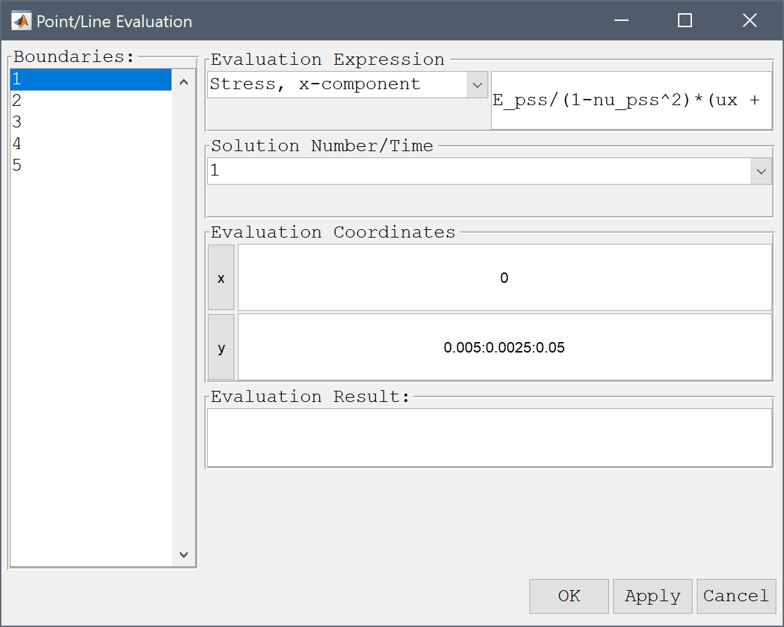
Press the Apply button to create the line plot.
load/2*(2+0.005^2/y^2+3*0.005^4/y^4) into the edit field.The thin plate with a hole structural mechanics model has now been completed and can be saved as a binary (.fea) model file, or exported as a programmable MATLAB m-script text file (available as the example ex_planestress1 script file), or GUI script (.fes) file.
[1] Kirsch EG, Die Theorie der Elastizitaet und die Beduerfnisse der Festigkeitslehre. Zeitschrift des Vereines deutscher Ingenieure, Vol. 42, pp. 797-807, 1898.