Cantilever Beam

A test case for a one dimensional model of a cantilever beam which is fixed to a wall at the left end. Using Euler-Bernoulli beam theory three test cases are studied for which reference solutions are available, a point load at the left end, a uniform distributed load, and the natural vibration modes and frequencies without load.

Tutorial

This model is available as an automated tutorial by selecting Model Examples and Tutorials... > Structural Mechanics > Cantilever Beam from the File menu. Or alternatively, follow the step-by-step instructions below.

1. To start a new model click the New Model toolbar button, or select New Model... from the File menu.
2. Select the 1D radio button.
3. Select the Euler-Bernoulli Beam physics mode from the Select Physics drop-down menu.
4. Press OK to finish the physics mode selection.

First define a line geometry with length 2 and a grid for the simulation.

1. Press the Create line Toolbar button.
2. Enter 2 into the Line geometry maximum x-coordinate edit field.
3. Press OK to finish and close the dialog box.
4. Switch to Grid mode by clicking on the corresponding Mode Toolbar button.
5. Press the Refine Toolbar button.
6. Switch to Equation mode by clicking on the corresponding Mode Toolbar button.
7. Enter 1 into the Density edit field.
8. Enter 6 into the Cross section area edit field.
9. Enter 3 into the Modulus of elasticity edit field.
10. Enter 4 into the Cross section moment of intertia edit field.
11. Press OK to finish the equation and subdomain settings specification.

Set up the point load on the right boundary.

1. Switch to Boundary mode by clicking on the corresponding Mode Toolbar button.
2. Select the Fixed displacement radio button.
3. Select 2 in the Boundaries list box.
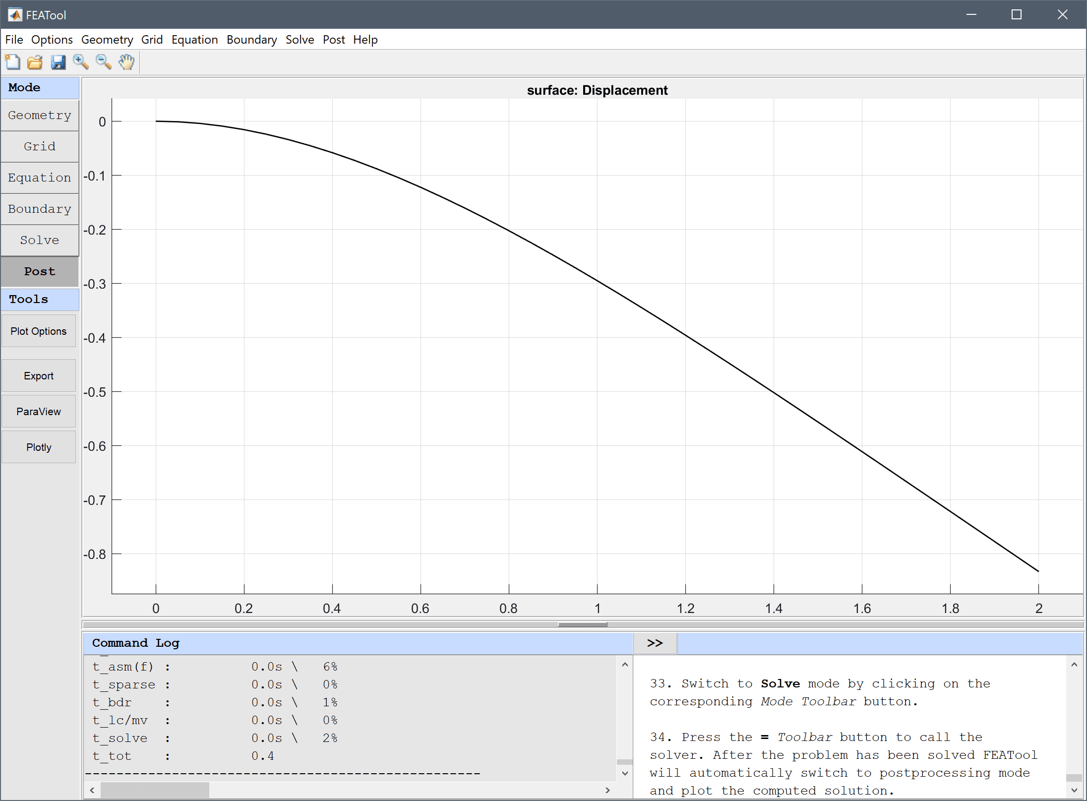
4. Enter -5 into the Displacement/load edit field.
5. Press OK to finish the boundary condition specification.
6. Switch to Solve mode by clicking on the corresponding Mode Toolbar button.
7. Press the = Toolbar button to call the solver. After the problem has been solved FEATool will automatically switch to postprocessing mode and plot the computed solution.

Verify that the maximum deflection at the end is equal to the analytical solution for a cantilever beam with a point load PL²/(3EI) = -1.1111.

1. Select Point/Line Evaluation... from the Post menu.
2. Enter 2 into the Evaluation coordinates in x-direction edit field.
3. Press the Apply button.
4. Press OK to finish and close the dialog box.

Go back to Equation mode to define a uniform load, and remove the point boundary condition load.

1. Enter -5 into the Distributed load/force edit field.
2. Press OK to finish the equation and subdomain settings specification.
3. Switch to Boundary mode by clicking on the corresponding Mode Toolbar button.
4. Select 2 in the Boundaries list box.
5. Enter 0 into the Displacement/load edit field.
6. Press OK to finish the boundary condition specification.
7. Switch to Solve mode by clicking on the corresponding Mode Toolbar button.
8. Press the = Toolbar button to call the solver. After the problem has been solved FEATool will automatically switch to postprocessing mode and plot the computed solution.

Verify that the maximum deflection at the end is equal to the analytical solution for a cantilever beam with a uniformly distributed load q*L⁴/(8EI) = -0.8333.

1. Select Point/Line Evaluation... from the Post menu.
2. Enter 2 into the Evaluation coordinates in x-direction edit field.
3. Press OK to finish and close the dialog box.

To conduct a eigenmode analysis, change to the corresponding solver in the Solver Settings dialog box.

1. Switch to Solve mode by clicking on the corresponding Mode Toolbar button.
2. Press the Settings Toolbar button.
3. Select Eigenvalue from the Solution and solver type drop-down menu.
4. Press the Solve button.

Verify that the frequencies of the four first vibration modes are close to the reference frequencies 0.198, 1.24, 3.472, and 6.803 Hz.

1. Press the Plot Options Toolbar button.
2. Select 1.54438 (0.197786 Hz) from the Available solutions/eigenvalues (frequencies) drop-down menu.
3. Press OK to plot and visualize the selected postprocessing options.

The cantilever beam structural mechanics model has now been completed and can be saved as a binary (.fea) model file, or exported as a programmable MATLAB m-script text file (available as the example ex_euler_beam1 script file), or GUI script (.fes) file.