The classic Poisson equation is one of the most fundamental partial differential equations (PDEs). Although one of the simplest equations, it is a very good model for the process of diffusion and comes up again and again in many applications such as in fluid flow, heat transfer, and chemical transport.

This example shows how to set up and solve the Poisson equation

\[ d_{ts}\frac{\partial u}{\partial t} + \nabla\cdot(-D\nabla u) = f \]

for a scalar field u = u(x) on a circle with radius r = 1. The diffusion coefficient D = 1 and right hand side source term f = δ(0,0) which prescribes a point source at the center. The Poisson problem is also considered stationary meaning that time dependent term can be neglected. With these assumptions the equation simplifies to

\[ - \Delta u = \delta(0,0). \]

Moreover, homogeneous Dirichlet boundary conditions are prescribed on all boundaries of the domain, that is u = 0 on the boundary. The exact solution for this problem is u(x,y) = -1/(2*π)*log( r ) and can be used to measure the accuracy of the computed solution.

Tutorial

How to set up and solve the Poisson equation (1) with the FEATool graphical user interface (GUI) is described in the following. Alternatively, this tutorial example can also be automatically run by selecting it from the File > Model Examples and Tutorials > Quickstart menu, or viewed as a video tutorial.

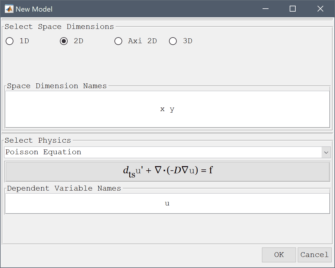
Start MATLAB and launch FEATool by clicking on the corresponding icon in the MATLAB Add-Ons toolbar (or type featool on the command line from the installation directory when not using FEATool as an installed toolbox).
To start a new model click the New Model toolbar button, or select New Model... from the File menu.

In the New Model dialog box, select 2D for the Space Dimensions, and select Poisson Equation from the Select Physics drop-down menu. Leave the space dimension and dependent variable names to their defaults and press OK to finish the physics mode selection.
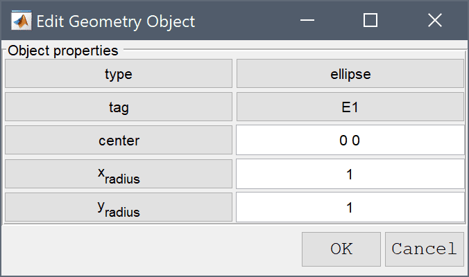
To create a circle or ellipse, first click on the Create circle/ellipse Toolbar button. Then left click in the main plot axes window, and hold down the mouse button. Move the mouse pointer to draw the shape outline, and release the button to finalize the shape.
The object properties must be changed to make a unit circle with radius 1 centered at the origin (0, 0). To do this, click on the ellipse E1 to select it and highlight it (alternatively select it by clicking on E1 in the left side toolbar selection list box). Then click on the Inspect/edit selected geometry object Toolbar button.
In the Edit Geometry Object dialog box change the center coordinates edit field to 0 0, and set both the x and y-radius to 1. Finish editing the geometry object and close the dialog box by clicking OK.

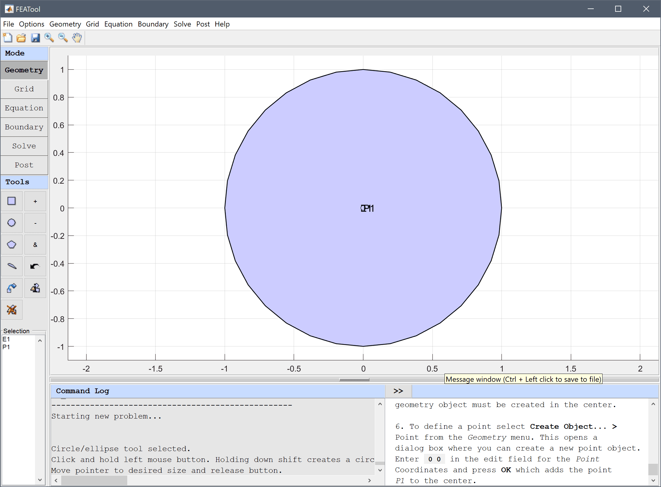
To make sure that a grid point for the source term will be located exactly at (0, 0), a point geometry object must be created in the center.

To define a point select Create Object... > Point from the Geometry menu. This opens a dialog box where you can create a new point object. Enter 0 0 in the edit field for the Point Coordinates and press OK which adds the point P1 to the center.
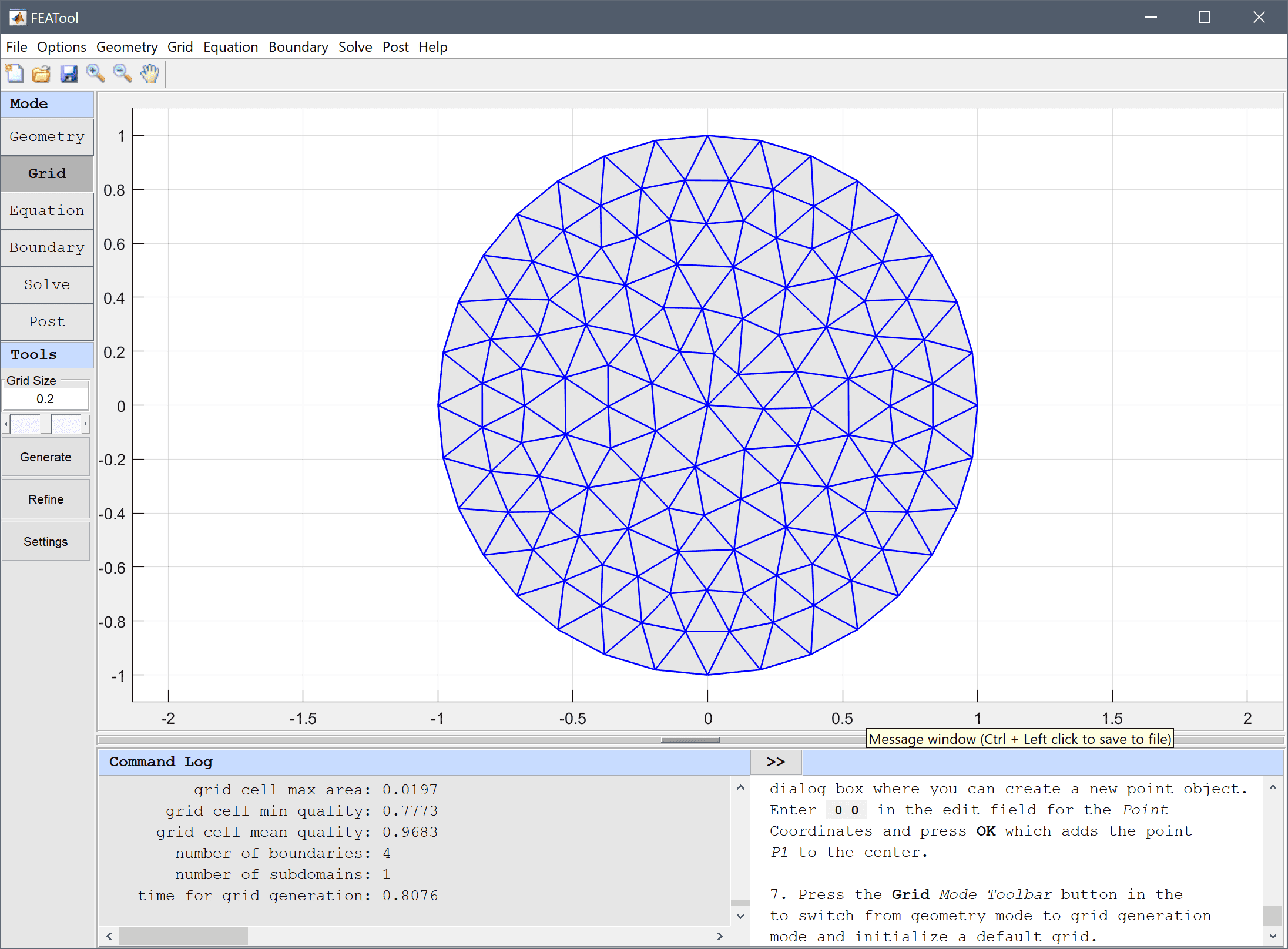
Press the Grid Mode Toolbar button to switch from geometry mode to grid generation mode and initialize a default grid.
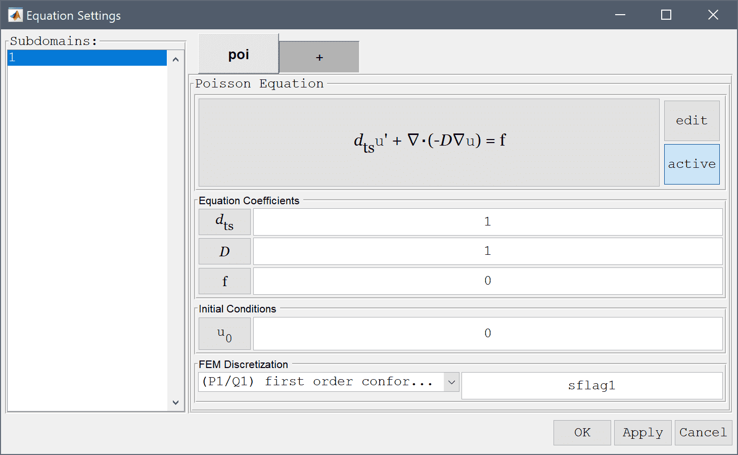
Switch to Equation mode by clicking on the corresponding Mode Toolbar button.
Equation and material coefficients can be specified in Equation/Subdomain mode. In the Equation Settings dialog box that automatically opens, set the diffusion coefficient D to 1 and source term f to 0 in the corresponding edit fields. All other coefficients can be left to their default values. Press OK to finish and close the dialog box.
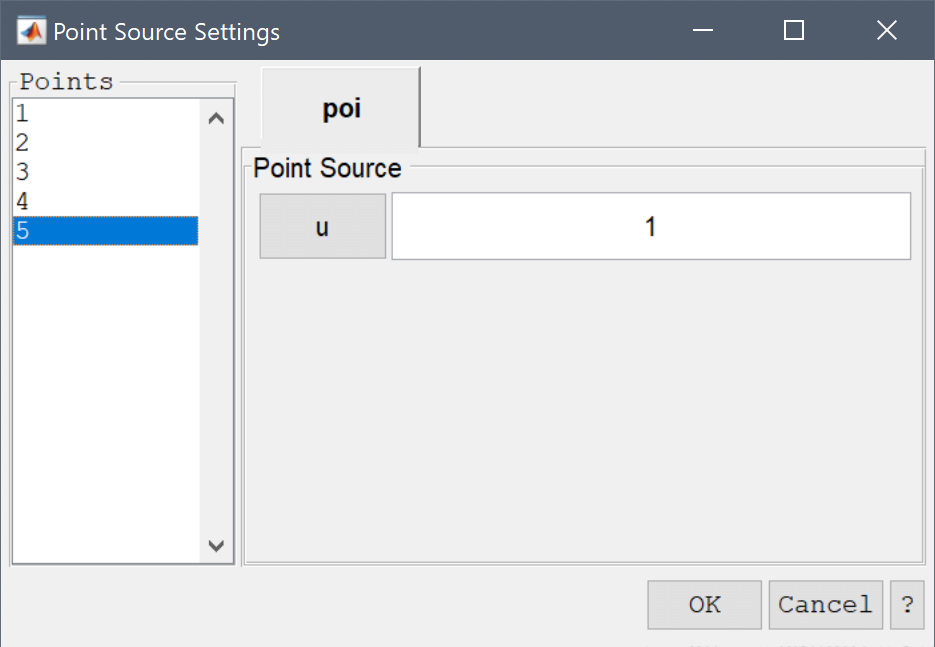
To add the point source, select Add Point Sources... from the Equation menu, and enter 1 in the corresponding edit field for the center point (point number 5). Press OK to finish.
Switch to Boundary mode by clicking on the corresponding Mode Toolbar button.
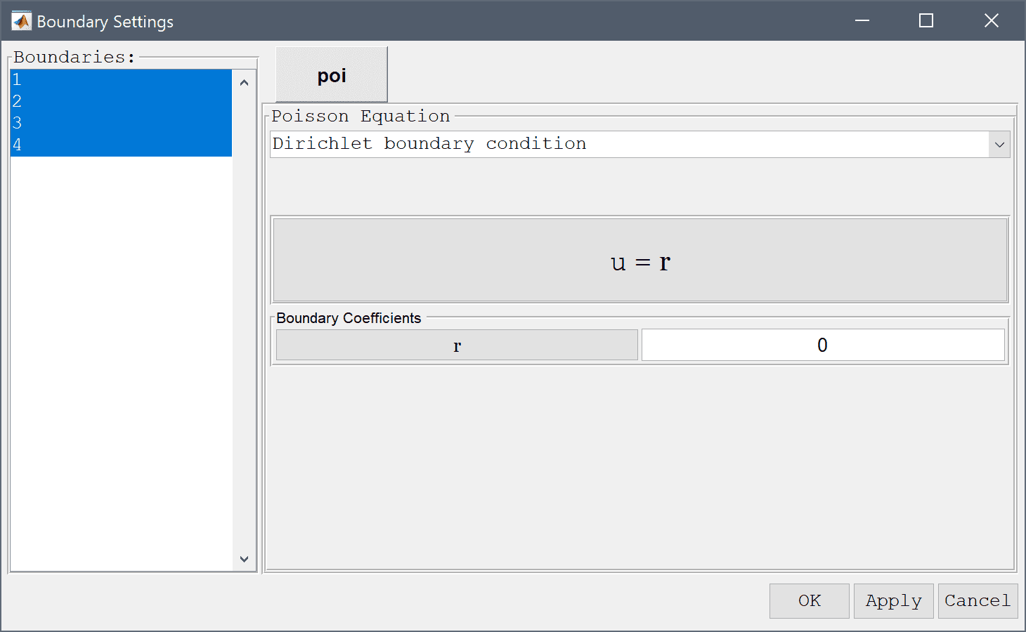
In the Boundary Settings dialog box, select all boundaries in the left hand side Boundaries list box, and choose Dirichlet boundary condition in the drop-down menu. Set the Dirichlet boundary coefficient r equal to 0, and finish by clicking on OK.
Now that the problem is fully specified, press the Solve Mode Toolbar button to switch to solve mode. Then press the = Tool button to call the solver with the default solver settings.
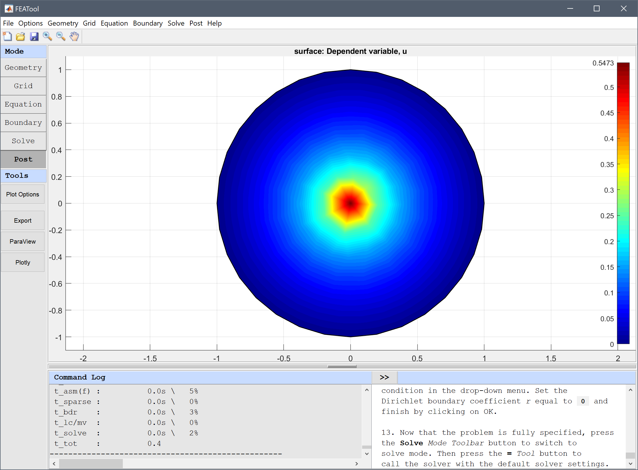
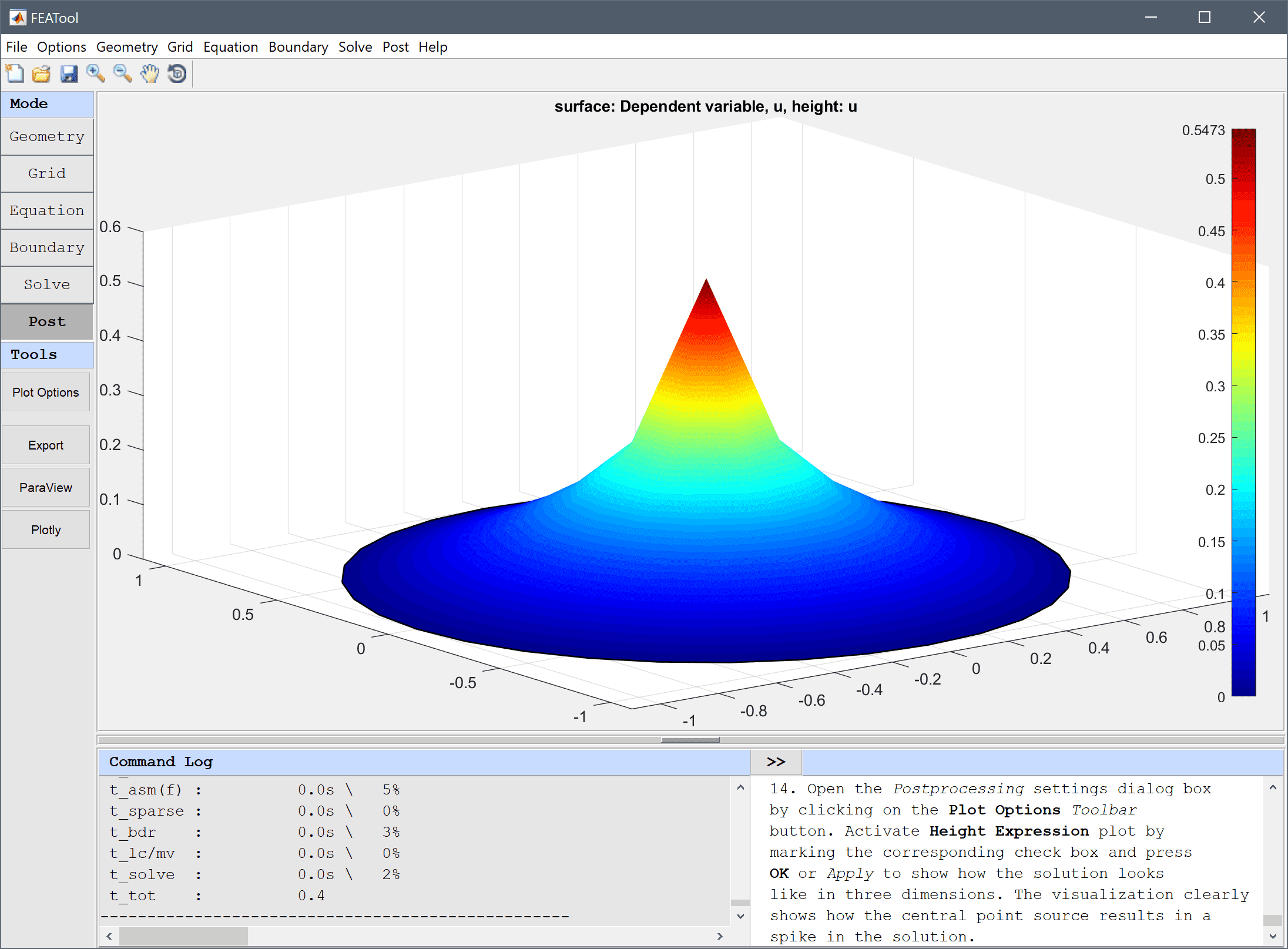
Open the Postprocessing settings dialog box by clicking on the Plot Options Toolbar button. To see how the solution looks like in three dimensions, activate Height Expression plot by marking the corresponding check box, and press OK or Apply. The resulting visualization clearly shows how the central point source results in a spike in the solution.
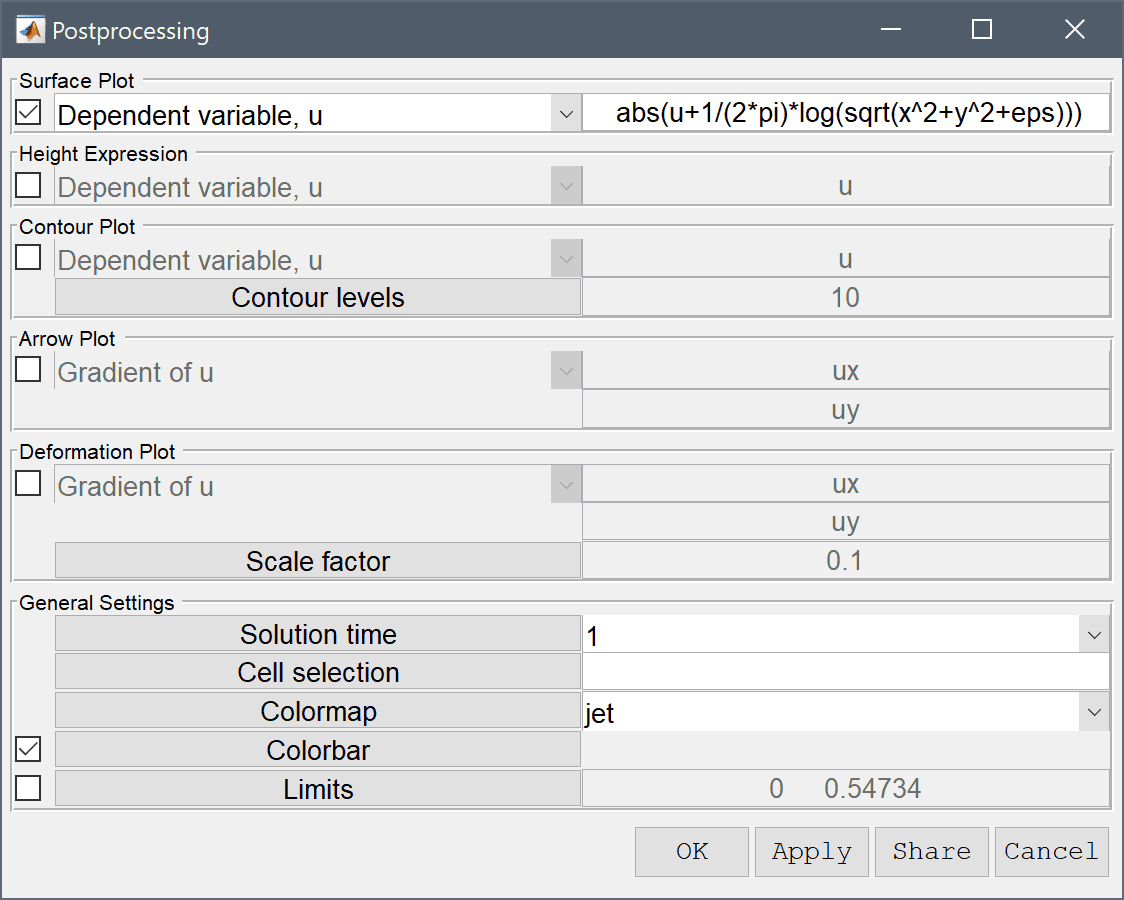
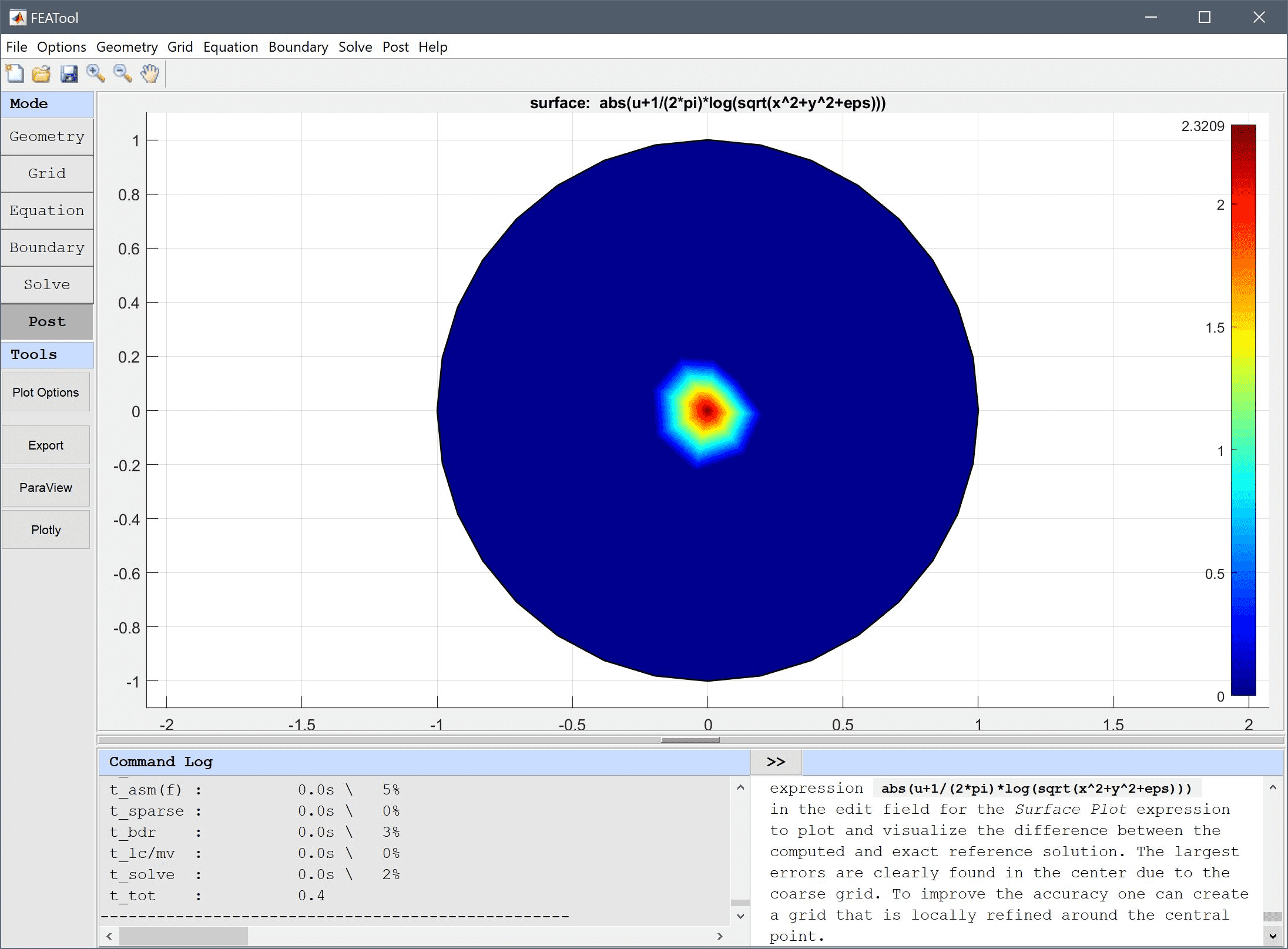
To plot and visualize the difference between the computed and exact reference solution, enter the analytical expression abs(u+1/(2*pi)*log(sqrt(x^2+y^2+eps))) in the edit field for the Surface Plot expression. The largest errors are clearly found in the center due to the coarse grid. To improve the accuracy one can create a grid that is locally refined around the central point.

The poisson equation with a point source classic pde model has now been completed and can be saved as a binary (.fea) model file, or exported as a programmable MATLAB m-script text file, (available as the example ex_poisson7 script file), or GUI script (.fes) file.

Tutorial

Video