This section explains how to set up and solve a generalized wave equation model. The wave equation is a hyperbolic partial differential equation (PDE) of the form

\[ \frac{\partial^2 u}{\partial t^2} = c\Delta u + f \]

where c is a constant defining the propagation speed of the waves, and f is a source term. This equation can not be solved as it is due to the second order time derivative. However, the problem can be transformed by reformulating the wave equation as two coupled parabolic PDEs, that is

\[ \left\{\begin{array}{l} \frac{\partial u}{\partial t} = v \\ \frac{\partial v}{\partial t} = c\Delta u + f \end{array}\right. \]

This dual coupled problem can easily be implemented in FEATool with the custom equation feature. This example solves the wave equation on a unit circle, with zero boundary conditions, constant c = 1, source term f = 0, and initial condition u(t=0) = 1 - ( x² + y² ).

Tutorial

How to set up and solve the wave equation with the FEATool graphical user interface (GUI) is described in the following. Alternatively, this tutorial example can also be automatically run by selecting it from the File > Model Examples and Tutorials > Quickstart menu, or viewed as a video tutorial.

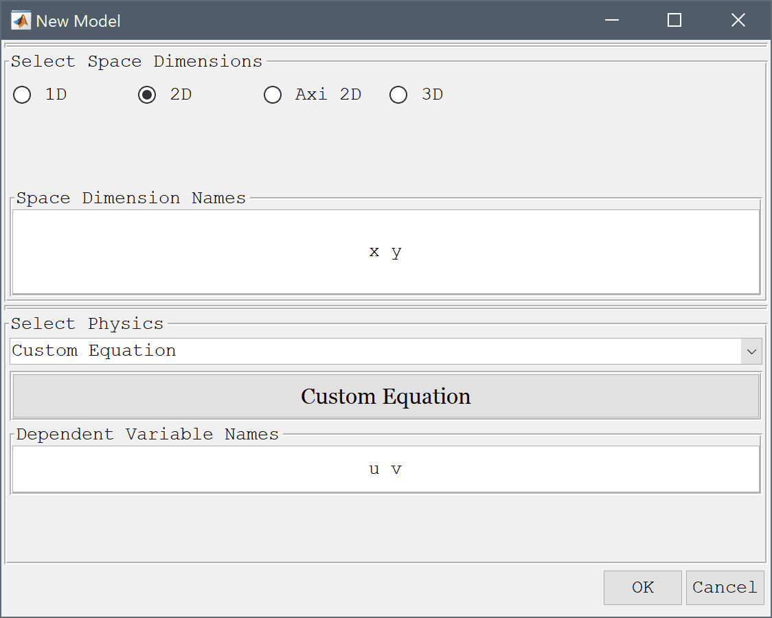
Start MATLAB and launch FEATool by clicking on the corresponding icon in the MATLAB Add-Ons toolbar (or type featool on the command line from the installation directory when not using FEATool as an installed toolbox).
To start a new model click the New Model toolbar button, or select New Model... from the File menu.
In the New Model dialog box, first click on the 2D radio button in the Select Space Dimensions section, and select Custom Equation from the Select Physics drop-down menu. Leave the space dimension names as x y, but change the dependent variable names to u v (the custom equation physics mode allows for entering an arbitrary number of dependent variables). This will enable the two parabolic equations for the transformed and coupled wave equation problem. Finish and close the dialog box by clicking on the OK button.

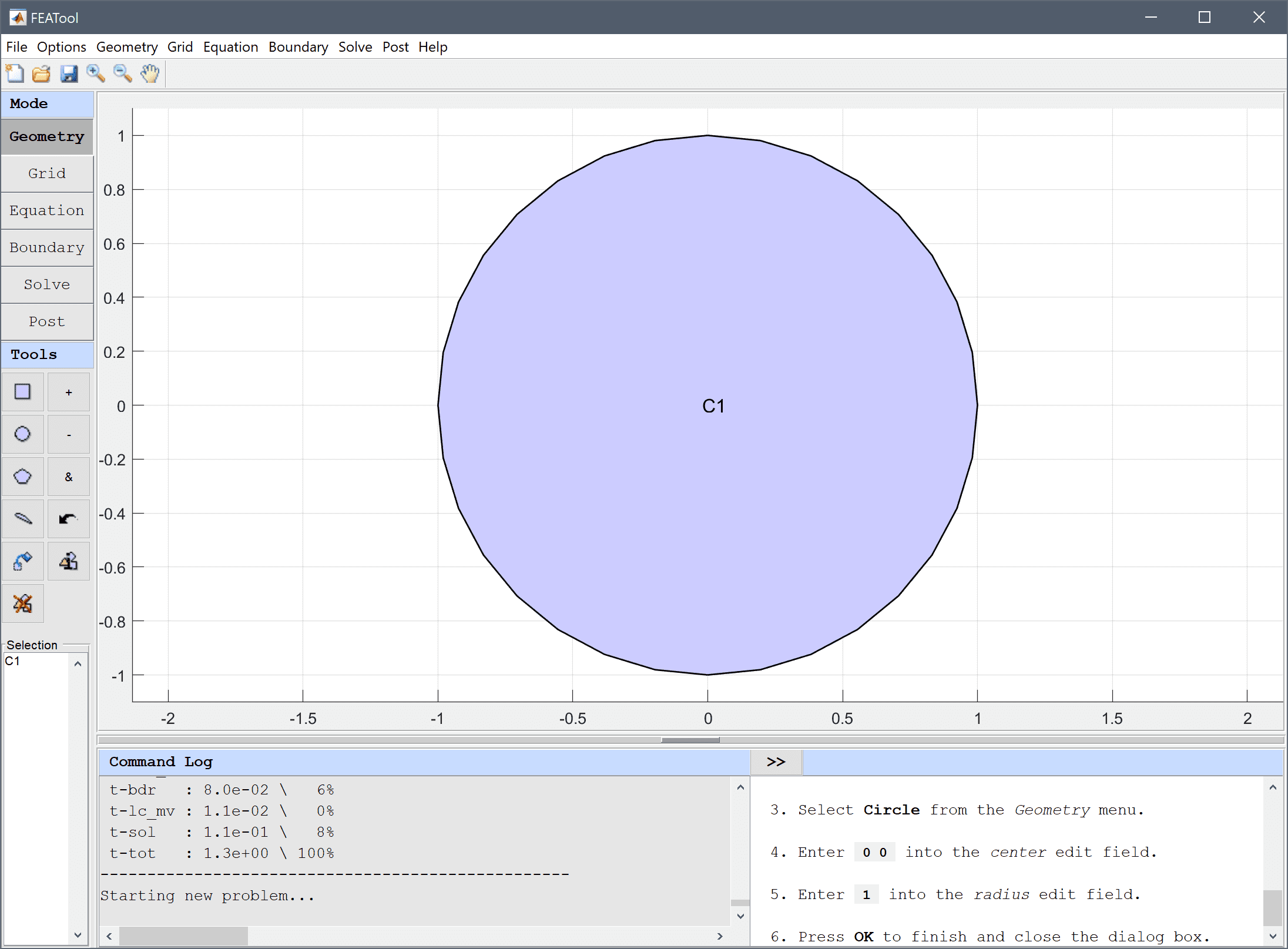
The geometry consists of a unit circle with radius 1 centered at the origin (0, 0).

Select Circle from the Geometry menu.
Enter 0 0 into the center edit field, and 1 into the radius edit field.
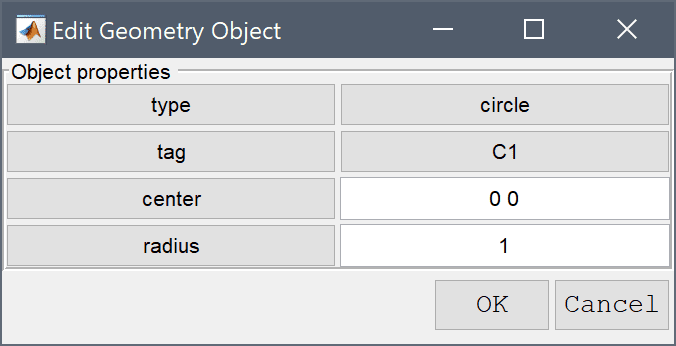
Press OK to finish and close the dialog box.
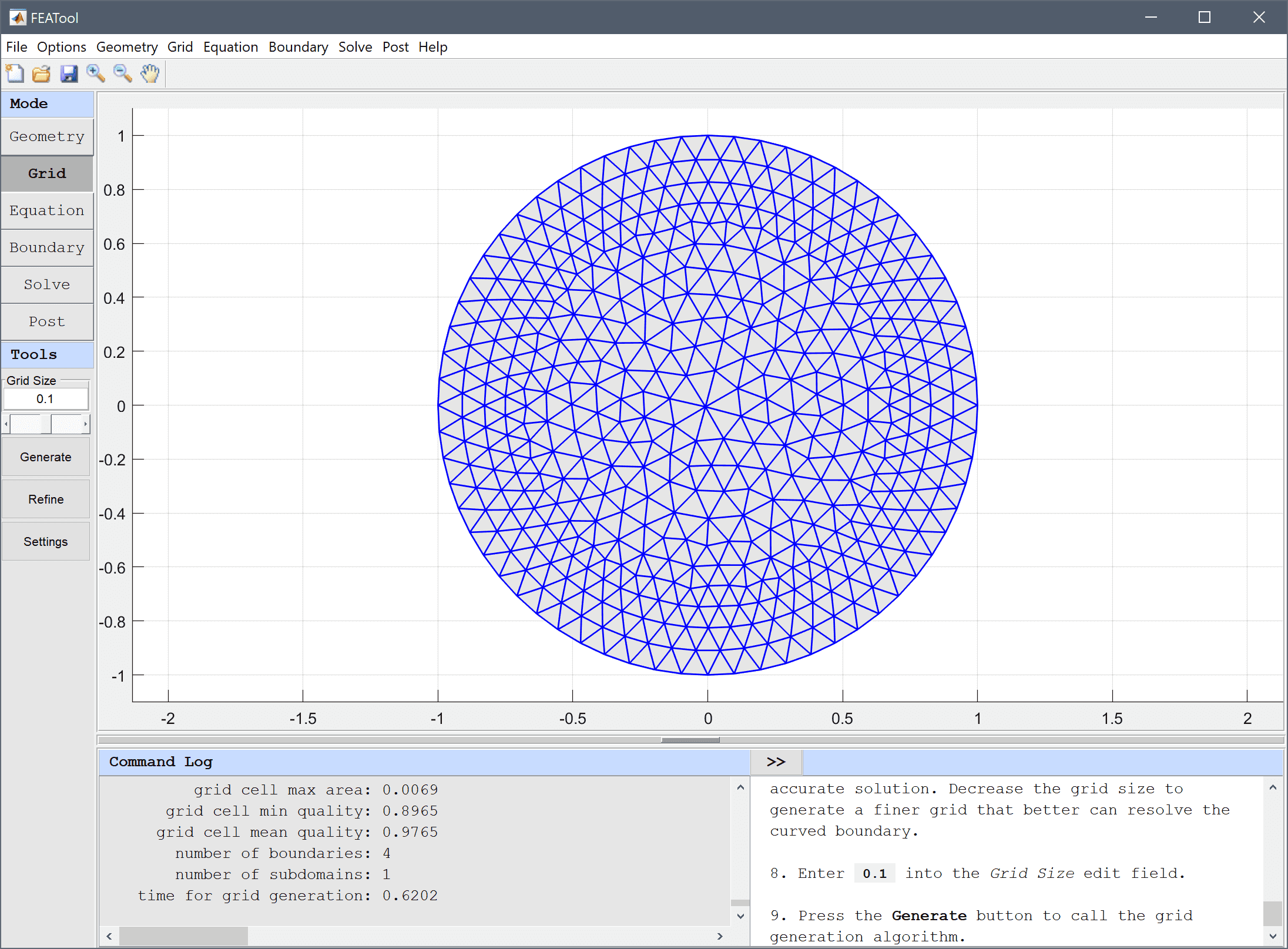
Switch to Grid mode by clicking on the corresponding Mode Toolbar button.

The default grid may be too coarse to ensure an accurate solution. Decrease the grid size to generate a finer grid which is able to resolve the curved boundary better.

Enter 0.1 into the Grid Size edit field, and press the Generate button to call the grid generation algorithm.
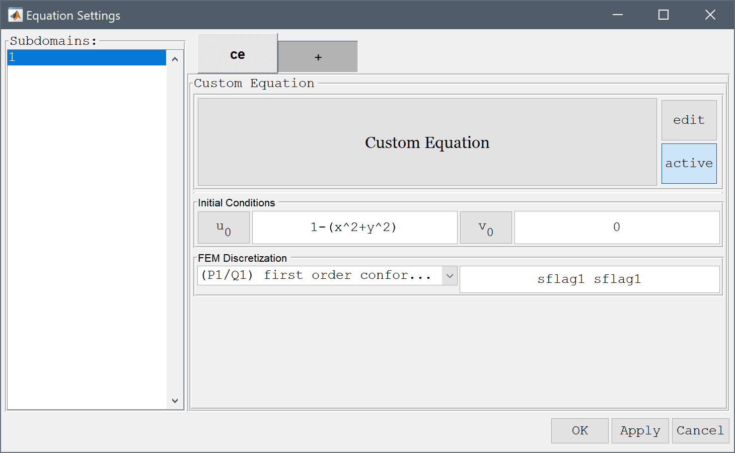
Switch to Equation mode by clicking on the corresponding Mode Toolbar button.
Equation and material coefficients are specified in Equation/Subdomain mode. Set the initial condition u0 to 1-(x^2+y^2) and v0 to 0. Then click on the edit button to open the equation editing dialog box.
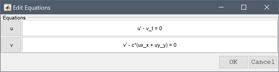
In the Edit Equations dialog box enter the two coupled equations as u' - v_t = 0, and v' - c*(ux_x + uy_y) = 0 in the corresponding edit fields for u and v.

Here u and v are the dependent variables, u'/v' denotes a time derivative, and an underscore will treat it implicitly in the weak finite element formulation (for example v_t corresponds to v multiplied with the test function for u, and ux_x is analogous to du/dx*dv_t/dx). Note, that the first equation could also be written as u' = v but then v would be evaluated explicitly in the right hand side, by transferring it to the implicit left hand side matrix results in a linear problem which is more efficient to solve.

![](wave_equation1_12_50.png)

Press OK to finish the equation and subdomain settings specification.

A convenient way to define and store coefficients, variables, and expressions is using the Model Constants and Expressions functionality. The defined expressions can then be used in point, equation, boundary coefficients, as well as postprocessing expressions, and can easily be changed and updated in a single place.

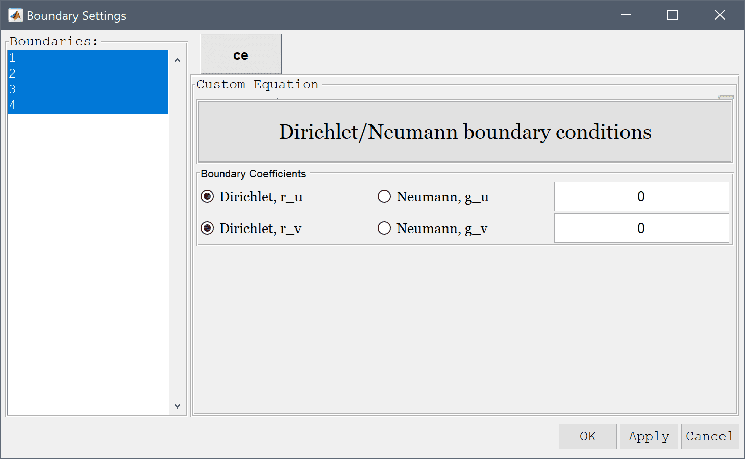
Click on the Constants Toolbar button and enter a new constant named c, with a value of 1 for the wave speed (this is the constant used in diffusion term of the second v equation). Press OK to finish.
Press the Boundary Mode Toolbar button to change to boundary condition specification mode, and select Dirichlet conditions with a fixed value of 0 for all boundaries.
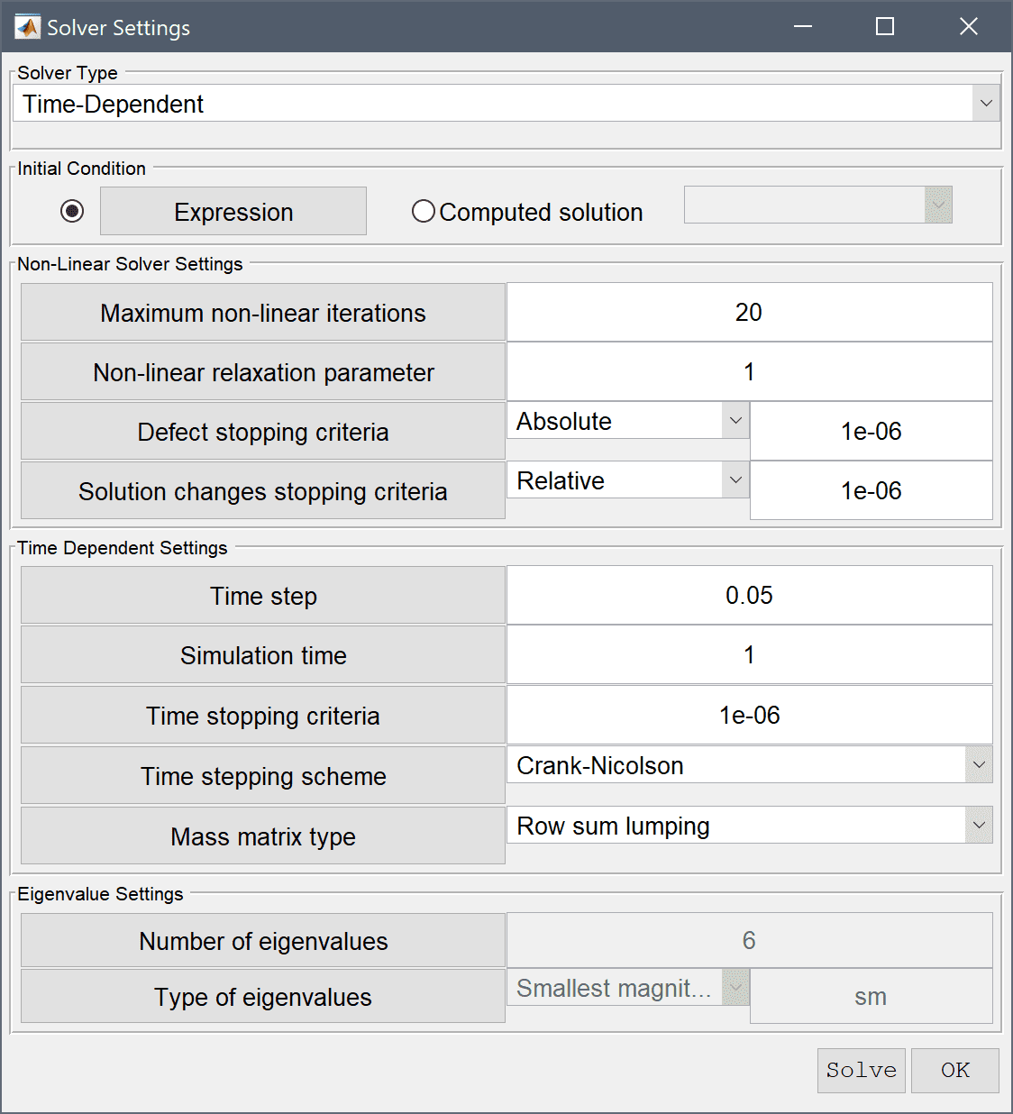
Switch to Solve mode by clicking on the corresponding Mode Toolbar button.
Press the Settings Toolbar button to open the Solver Settings dialog box, select the Time-Dependent Solver Type option, and set the Time step to 0.05
Press the Solve button to start the solver with the chosen settings, or press OK and then the = Toolbar button.

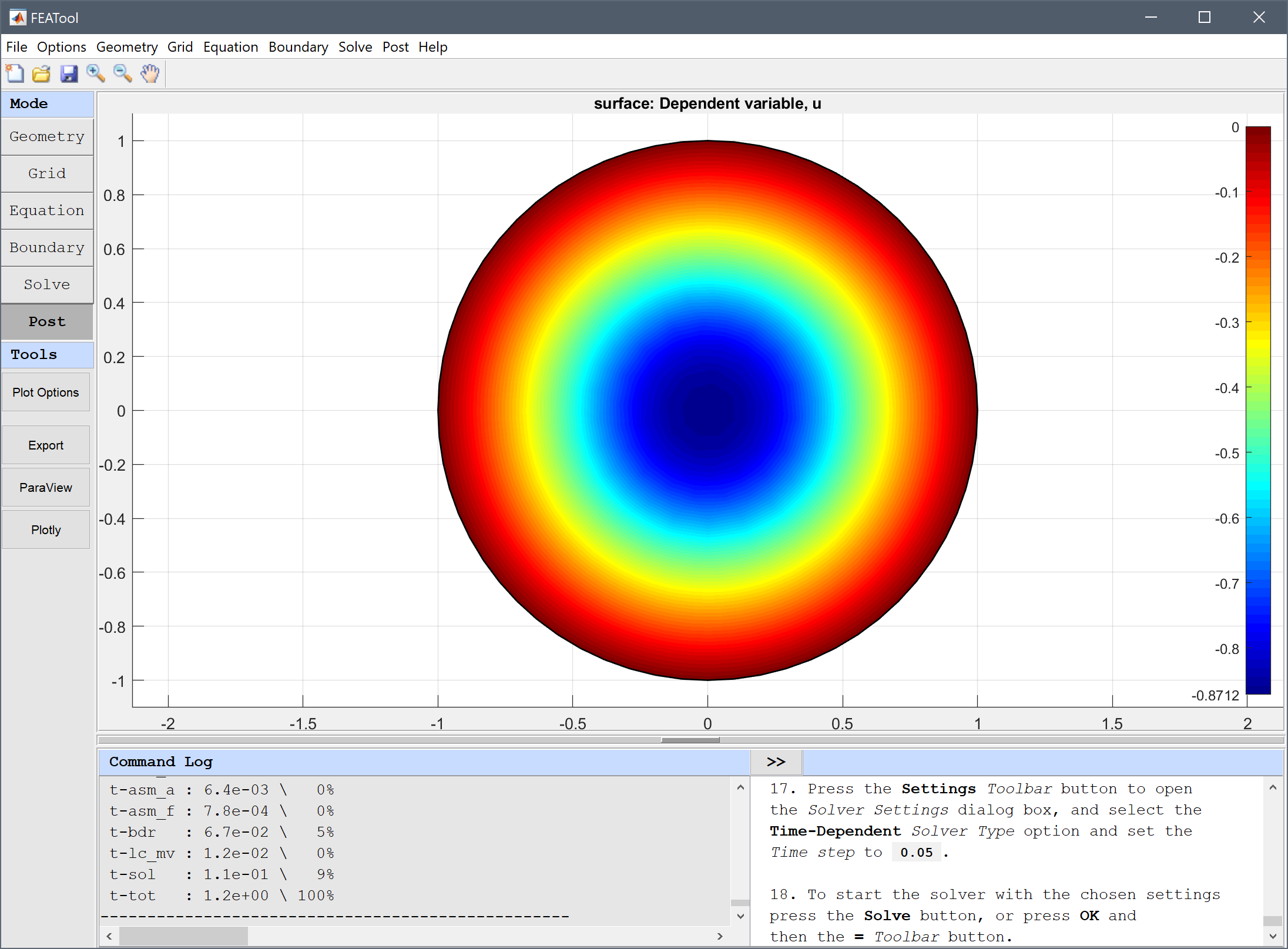
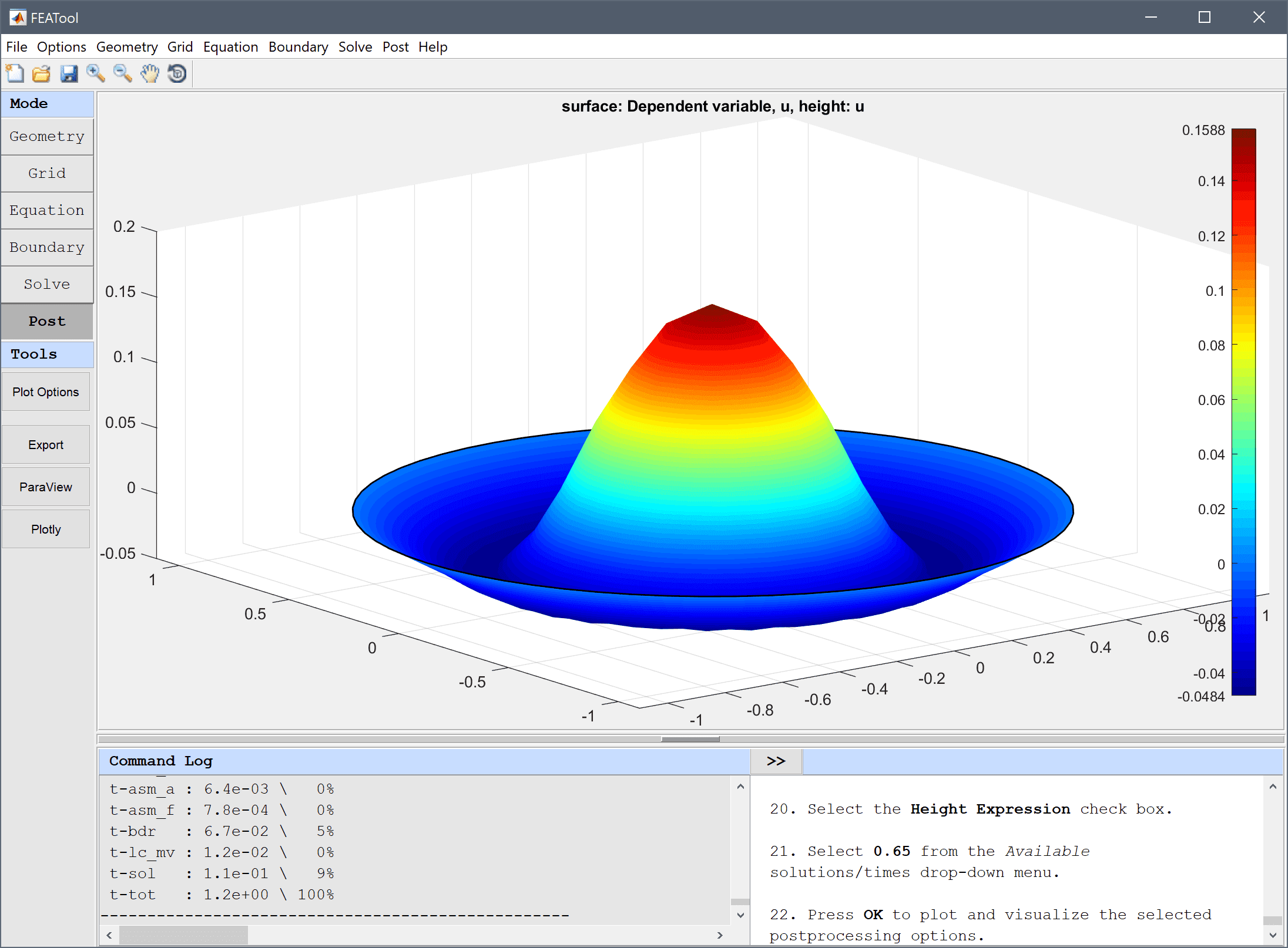
The solution at different time steps can be visualized by selecting the corresponding solution times, and plot options in the postprocessing settings dialog box.

Press the Plot Options Toolbar button.
Select the Height Expression check box.
Select 0.65 from the Available solutions/times drop-down menu.
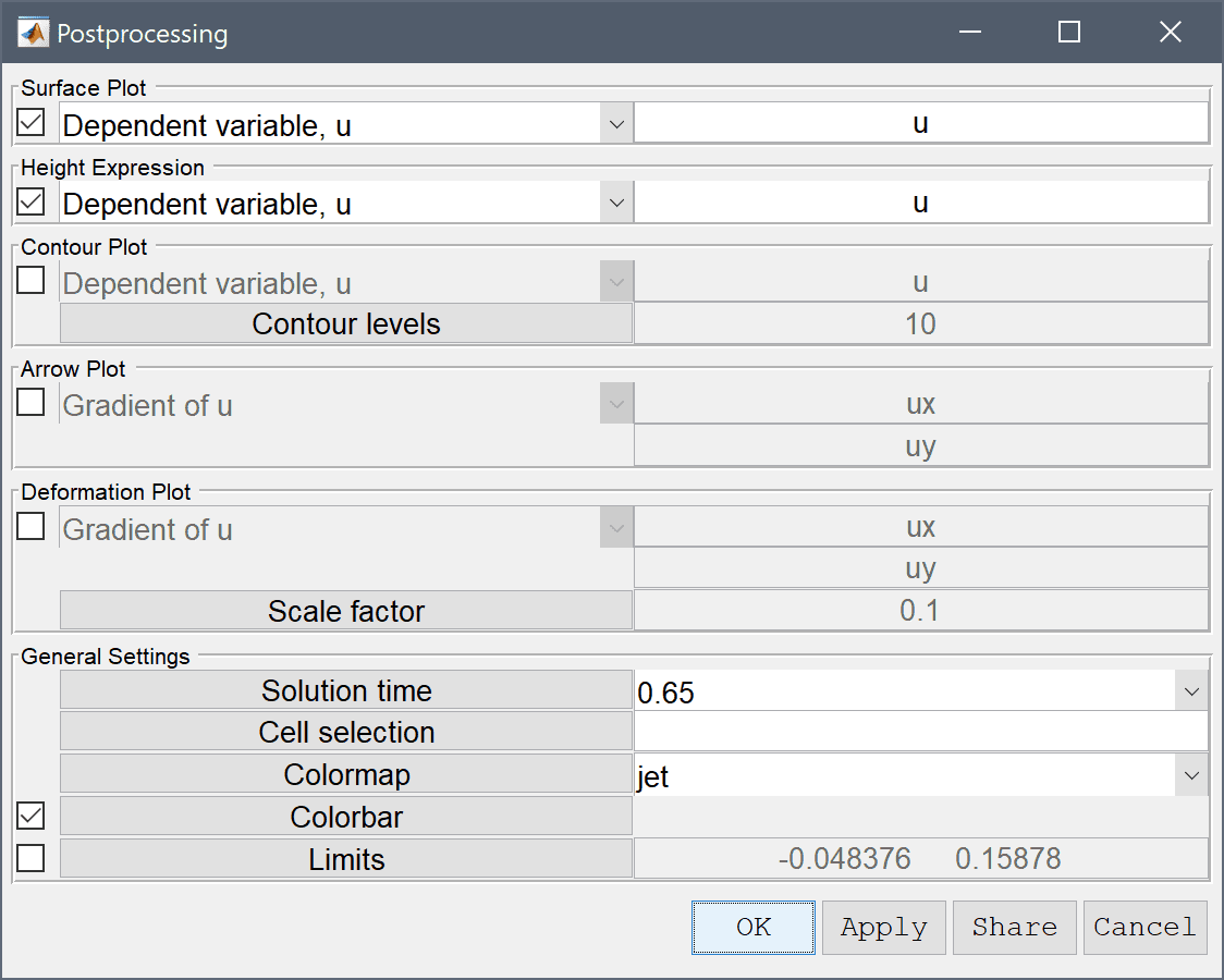
Press OK to plot and visualize the selected postprocessing options.

To create an animation or video of the solution one can use the Animate/Playback Solution... option in the Post menu.

The wave equation on a circle classic PDE model has now been completed and can be saved as a binary (.fea) model file, or exported as a programmable MATLAB m-script text file (available as the example ex_waveequation1 script file), or GUI script (.fes) file.

Tutorial

Video