Resonance Frequencies of a Room

This example studies the resonance frequencies of an empty room by using the Helmholtz equation for the time-harmonic pressure field

\[ \Delta p + k^2 p = 0 \]

The resulting eigenmodes can be compared to and validated against the analytical solution for the resonance frequencies of a boxed enclosure, that is f = c/2*√( (i/lx)² + (j/ly)² + (k/lz)² ) where i, j, and k are integer permutations 0 ... n for the various modes.

Tutorial

This model is available as an automated tutorial by selecting Model Examples and Tutorials... > Classic PDE > Resonance Frequencies of a Room from the File menu, and can be viewed as a video tutorial. Or alternatively, follow the step-by-step instructions below.

1. To start a new model click the New Model toolbar button, or select New Model... from the File menu.
2. Select the 3D radio button.

Both the Poisson Equation and Custom Equation physics modes are suitable starting points for this model example, but in the following tutorial the Custom Equation will be used.

1. Select the Custom Equation physics mode from the Select Physics drop-down menu.
2. Enter p into the Dependent Variable Names edit field.
3. Press OK to finish the physics mode selection.
4. Press the Create cube/block Toolbar button.
5. Enter 4 into the x_max edit field.
6. Enter 3 into the y_max edit field.
7. Enter 2.6 into the z_max edit field.
8. Press OK to finish and close the dialog box.
9. Switch to Grid mode by clicking on the corresponding Mode Toolbar button.
10. Enter 0.5 into the Grid Size edit field.
11. Press the Generate button to call the grid generation algorithm.
12. Switch to Equation mode by clicking on the corresponding Mode Toolbar button.
13. Press the edit button.

For this eigenmode analysis the right hand side of the Helmholtz equation is not involved and is therefore set to zero.

1. Enter p' - (px_x + py_y + pz_z) = 0 into the Equation for p edit field.
2. Press OK to finish and close the dialog box.
3. Press OK to finish the equation and subdomain settings specification.
4. Switch to Boundary mode by clicking on the corresponding Mode Toolbar button.

Homogeneous Neumann boundary conditions are used for all boundaries to represent solid and impermeable walls.

1. Select all boundaries (1-6) in the list box.
2. Select the Neumann, g_p radio button.
3. Press OK to finish the boundary condition specification.
4. Switch to Solve mode by clicking on the corresponding Mode Toolbar button.
5. Press the Settings Toolbar button.

Select the Eigenvalue solver in the Solver Settings dialog box, and increase the number of eigenmodes to compute to 9

1. Press the Solve button.

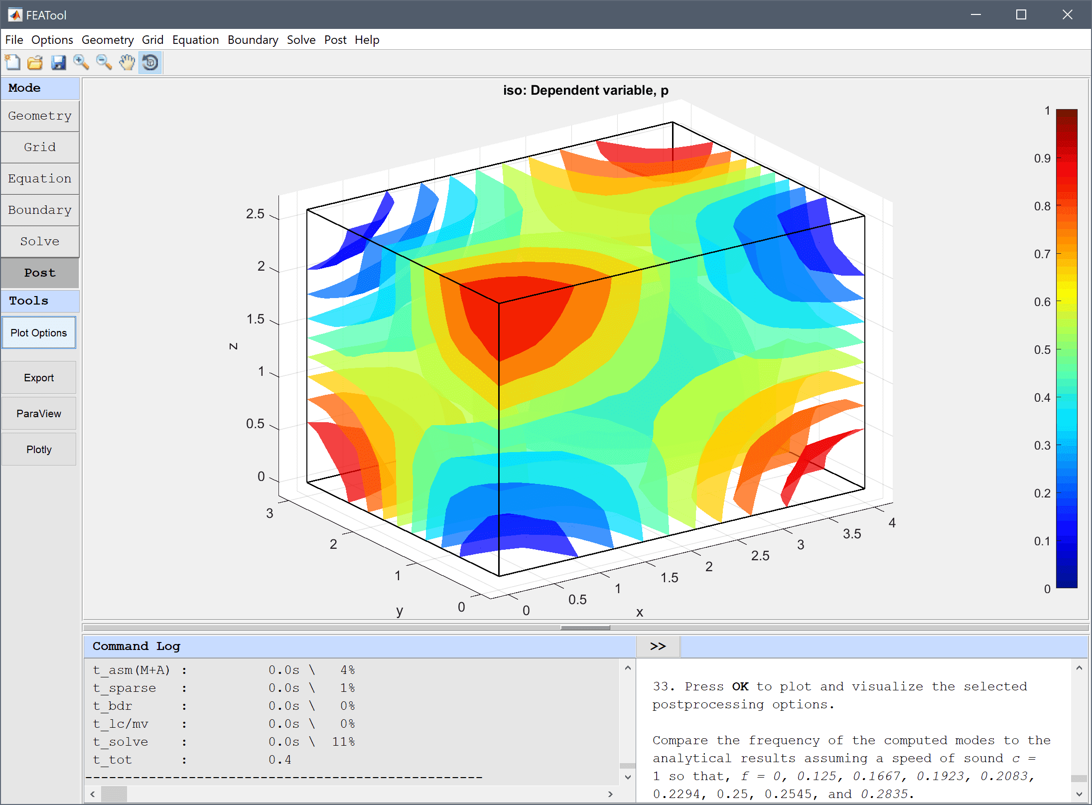
Open the Postprocessing settings dialog box, plot and visualize some eigenmodes to compare them. One can see how the lower modes resonate in a single direction, and increase in complexity and frequency as the number of resonance modes are added.

1. Press the Plot Options Toolbar button.
2. Clear the Surface Plot check box.
3. Select the Iso Plot check box.
4. Press Apply to plot and visualize the selected postprocessing options.
5. Select 0.611429 (0.124449 Hz) from the Available solutions/eigenvalues (frequencies) drop-down menu.
6. Press Apply to plot and visualize the selected postprocessing options.
7. Select 1.07499 (0.165015 Hz) from the Available solutions/eigenvalues (frequencies) drop-down menu.
8. Press OK to plot and visualize the selected postprocessing options.

Compare the frequency of the computed modes to the analytical results assuming a speed of sound c = 1 so that, f = 0, 0.125, 0.1667, 0.1923, 0.2083, 0.2294, 0.25, 0.2545, and 0.2835.

The resonance frequencies of a room classic PDE model has now been completed and can be saved as a binary (.fea) model file, or exported as a programmable MATLAB m-script text file, or GUI script (.fes) file.

Video