Shallow Water Equations

Saint-Venant shallow water equations is a simplified model of fluid flow with a free surface. The non-conservative form of the equations read

\[ \left\{\begin{array}{l} \frac{\partial h}{\partial t} + (u\frac{\partial h}{\partial x} + v\frac{\partial h}{\partial y} ) + (h+H)(\frac{\partial u}{\partial x} + \frac{\partial v}{\partial y}) = 0 \\ \frac{\partial u}{\partial t} + (u\frac{\partial u}{\partial x} + v\frac{\partial u}{\partial y} ) = -g\frac{\partial h}{\partial x} \\ \frac{\partial v}{\partial t} + (u\frac{\partial v}{\partial x} + v\frac{\partial v}{\partial y} ) = -g\frac{\partial h}{\partial y} \end{array}\right. \]

where h is the unknown free surface height relative to the mean level H.

Tutorial

This model is available as an automated tutorial by selecting Model Examples and Tutorials... > Classic PDE > Shallow Water Equations from the File menu, viewed as a videotutorial", or alternatively, follow the step-by-step instructions below.

1. To start a new model click the New Model toolbar button, or select New Model... from the File menu.

Both the Custom Equation and Convection and Diffusion physics modes are used in this example.

1. Select the Custom Equation physics mode from the Select Physics drop-down menu.
2. Enter h into the Dependent Variable Names edit field.
3. Press OK to finish the physics mode selection.
4. Select Rectangle from the Geometry menu.
5. Enter 0 into the x_min edit field.
6. Enter 5 into the x_max edit field.
7. Enter 0 into the y_min edit field.
8. Enter 1 into the y_max edit field.
9. Press OK to finish and close the dialog box.
10. Switch to Grid mode by clicking on the corresponding Mode Toolbar button.
11. Enter 0.2 into the Grid Size edit field.
12. Press the Generate button to call the grid generation algorithm.
13. Switch to Equation mode by clicking on the corresponding Mode Toolbar button.
14. Press the edit button.
15. Enter the equation for the surface height, h' + (u*hx_t + v*hy_t) + (h+H)*(ux_t+vy_t) = 0, into the edit field for the h equation.
16. Press OK to finish and close the dialog box.
17. An initial small disturbance, or height difference, is required to see any wave phenomena. Enter 0.2*exp(-((x-4)^2)) into the edit field for the Initial condition for h.

Now add two Convection and Diffusion physics modes for the horizontal velocity components u and v. Although the Custom Equation physics mode could also be used here, the Convection and Diffusion physics modes feature pre-defined equations, and convective stabilization which is necessary here.

1. Switch to the + tab.
2. Select the Convection and Diffusion physics mode from the Select Physics drop-down menu.
3. Enter u into the Dependent Variable Names edit field.
4. Press the Add Physics >>> button.
5. Enter 0 into the Diffusion coefficient edit field.
6. Enter u into the Convection velocity in x-direction edit field.
7. Enter v into the Convection velocity in y-direction edit field.
8. Enter -g*hx into the Reaction rate edit field.
9. Press the Artificial Stabilization button.
10. Select the Check to enable shock capturing check box.
11. Select High order from the Shock capturing discretization order drop-down menu.
12. Press OK to finish and close the dialog box.
13. Switch to the + tab.
14. Select the Convection and Diffusion physics mode from the Select Physics drop-down menu.
15. Enter v into the Dependent Variable Names edit field.
16. Press the Add Physics >>> button.
17. Enter 0 into the Diffusion coefficient edit field.
18. Enter u into the Convection velocity in x-direction edit field.
19. Enter v into the Convection velocity in y-direction edit field.
20. Enter -g*hy into the Reaction rate edit field.
21. Press the Artificial Stabilization button.
22. Select the Check to enable shock capturing check box.
23. Select High order from the Shock capturing discretization order drop-down menu.
24. Press OK to finish and close the dialog box.
25. Press OK to finish the equation and subdomain settings specification.

Two constants also have to be defined, one for the mean fluid level H = 1, and one for the gravitational constant g = 9.8.

1. Switch to Boundary mode by clicking on the corresponding Mode Toolbar button.

The height h should not be constrained, and should therefore be prescribed with homogeneous Neumann conditions everywhere.

1. Select all boudaries (1-4) in the Boundaries list box.
2. Select the Neumann, g_h radio button.

The right boundary is assumed to be a wall, and zero velocities are therefore prescribed there. The top and bottom boundaries are assumed to be symmetric, and feature zero flow in the normal direction.

1. Switch to the cd tab.
2. Select 4 in the Boundaries list box.
3. Select Concentration from the Convection and Diffusion drop-down menu.
4. Switch to the cd2 tab.
5. Select 1, 3, and 4 in the Boundaries list box.
6. Select Concentration from the Convection and Diffusion 2 drop-down menu.
7. Press OK to finish the boundary condition specification.
8. Switch to Solve mode by clicking on the corresponding Mode Toolbar button.
9. Press the Settings Toolbar button.

Select the Time-Dependent solver with the following parameters.

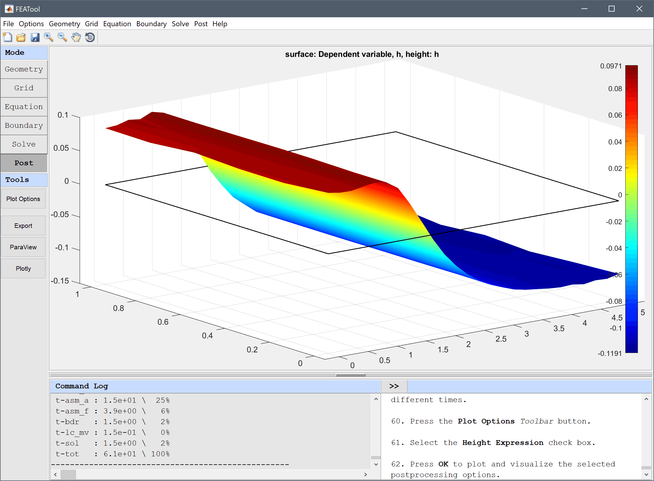
1. Enter 0.001 into the Non-linear stopping criteria for solution differences (changes) between iterations edit field.
2. Enter 0.01 into the Time step size edit field.
3. Enter 1.5 into the Duration of time-dependent simulation (maximum time) edit field.
4. Press the Solve button.

Once the solver has finished, turn on the height plot for h and visualize the free surface for different times.

1. Press the Plot Options Toolbar button.
2. Select the Height Expression check box.
3. Press OK to plot and visualize the selected postprocessing options.

One can also use the Animate/Playback Solution... option in the Post menu, to create an animation or video of the solution.

The shallow water equations fluid dynamics model has now been completed and can be saved as a binary (.fea) model file, or exported as a programmable MATLAB m-script text file, or GUI script (.fes) file.

Video