Potential Flow Over an Airfoil

Calculation of the inviscid flow field around a NACA airfoil using the potential equation. The potential or Laplace equation is equivalent to Poisson equation with a zero source term. Boundary conditions are set as zero normal flow on the airfoil body, and unit velocity magnitude at the external boundaries of the domain.

Tutorial

This model is available as an automated tutorial by selecting Model Examples and Tutorials... > Fluid Dynamics > Potential Flow Over an Airfoil from the File menu, viewed as a video tutorial, or alternatively, follow the step-by-step instructions below.

1. To start a new model click the New Model toolbar button, or select New Model... from the File menu.
2. Select the Poisson Equation physics mode from the Select Physics drop-down menu.
3. Enter phi into the Dependent Variable Names edit field.
4. Press OK to finish the physics mode selection.
5. Press the Create NACA airfoil Toolbar button.
6. Enter 0012 into the series edit field.
7. Enter 0 into the angle edit field.
8. Enter 100 into the resolution edit field.
9. Press OK to finish and close the dialog box.
10. To create a circle or ellipse, first click on the Create circle/ellipse Toolbar button. Then left click in the main plot axes window, and hold down the mouse button. Move the mouse pointer to draw the shape outline, and release the button to finalize the shape.
11. Select E1 in the geometry object Selection list box.
12. To modify and edit the selected ellipse, click on the Inspect/edit selected geometry object Toolbar button to open the Edit Geometry Object dialog box.
13. Enter 0.5 0 into the center edit field.
14. Enter 1.5 into the x_radius edit field.
15. Enter 1.5 into the y_radius edit field.
16. Press OK to finish and close the dialog box.
17. Select E1 and N1 in the geometry object Selection list box.
18. Press the - / Subtract geometry objects Toolbar button.
19. Switch to Grid mode by clicking on the corresponding Mode Toolbar button.
20. The default grid may be too coarse to ensure an accurate solution. Press the Settings button to open the Grid Settings dialog box, and select the Gridgen2D grid generation algorithm.
21. To fine tune the settings, enter 0.3 in the Subdomain Grid Size edit field and 0.3 0.3 0.3 0.3 0.05 0.05 for the Boundary Grid Size. This will ensure that the airfoil boundaries are resolved with fine grid cells, while the rest of the domain uses a coarse grid.
22. Also select the Boundary layers checkbox. This will create structured and higher quality grid cells near the airfoil boundaries.
23. Press the Generate button to call the grid generation algorithm.
24. Press OK to finish and close the dialog box.
25. Switch to Equation mode by clicking on the corresponding Mode Toolbar button.
26. Here the Poisson physics mode is used to model the equation for potential flow. In the Equation Settings dialog box, set the source term coefficient f to 0, and also select (P2/Q2) second order conforming for the FEM Discretization order to ensure that the velocities (which are derivatives of the potential) are represented with high accuracy.

A convenient way to define and store coefficients, variables, and expressions is using the Model Constants and Expressions functionality. The defined expressions can then be used in point, equation, boundary coefficients, as well as postprocessing expressions, and can easily be changed and updated in a single place.

1. Define expressions for the velocities, angle of attack, as well as pressure coefficient by pressing the Constants Toolbar button, or selecting the corresponding entry from the Equation menu, and entering the following variables in the Model Constants and Expressions dialog box. Press Enter after the last expression or use the Add Row button to expand the expression list.

Name	Expression
u	phix
v	phiy
U	sqrt(u^2+v^2)
alfa	0
uinf	cos(alfa*pi/180)
vinf	sin(alfa*pi/180)
cp	1-U^2/(uinf^2+vinf^2)

1. Switch to Boundary mode by clicking on the corresponding Mode Toolbar button.

For potential flow normal velocities can naturally be prescribed as Neumann boundary conditions. Set the flow at the exterior boundaries to nx*uinf+ny*uinf, and airfoil boundaries to zero (where nx and ny will be evaluated as the unit normal vectors of the boundaries).

1. Select the outer boundaries (1-4) in the Boundaries list box.
2. Select Neumann boundary condition from the Poisson Equation drop-down menu.
3. Enter nx*uinf+ny*vinf into the Neumann coefficient edit field.
4. Select the airfoil boundaries, 5 and 6, in the Boundaries list box.
5. Select Neumann boundary condition from the Poisson Equation drop-down menu.
6. Enter 0 into the Neumann coefficient edit field.
7. Press OK to finish the boundary condition specification.

One also has to set a reference level for the potential phi at one of the points, in order to ensure a unique solution for stationary problems without any Dirichlet/prescribed value boundary conditions.

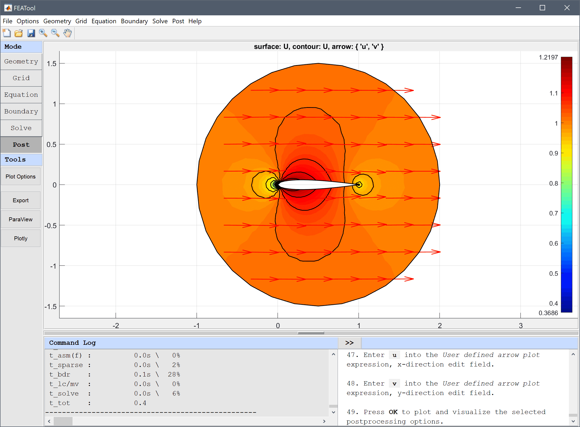
1. Select Add Point Constraints... from the Boundary menu.
2. Enter 0 into the edit field for the point at the trailing edge.
3. Press OK to finish and close the dialog box.
4. Switch to Solve mode by clicking on the corresponding Mode Toolbar button.
5. Press the = Toolbar button to call the solver. After the problem has been solved FEATool will automatically switch to postprocessing mode and plot the computed solution.

The potential function is displayed by default. Open the Postprocessing settings dialog box and visualize the velocity field U as surface, contour, and arrow plots instead.

1. Press the Plot Options Toolbar button.
2. Enter U into the User defined surface plot expression edit field.
3. Select the Contour Plot check box.
4. Enter U into the User defined contour plot expression edit field.
5. Enter 20 into the Number or specified vector of contour levels to plot edit field.
6. Select the Arrow Plot check box.
7. Enter u into the User defined arrow plot expression, x-direction edit field.
8. Enter v into the User defined arrow plot expression, y-direction edit field.
9. Press OK to plot and visualize the selected postprocessing options.

Use the Point/Line Evaluation functionality to plot the pressure coefficient cp along the upper wing boundary. At the stagnation point at the left edge the pressure coefficient should be close to 1, it then rapidly jumps towards -0.5 as the flow quickly accelerates, after which it slowly increases towards the trailing edge.

1. Select Point/Line Evaluation... from the Post menu.
2. Select 6 in the Boundaries list box.
3. Enter cp into the edit field.
4. Press OK to finish and close the dialog box.

To see how a higher angle of attack effects the flow field, change the previously defined constant alfa and solve the model again.

1. Select Model Constants and Expressions... from the Equation menu.
2. Enter 6 degrees into the expression edit field for the angle of attack, alfa.
3. Press OK to finish and close the dialog box.
4. Switch to Solve mode by clicking on the corresponding Mode Toolbar button.
5. Press the = Toolbar button to call the solver. After the problem has been solved FEATool will automatically switch to postprocessing mode and plot the computed solution.

Note that the flow field now is unsymmetric with two stagnation points. As the viscosity and the Kutta condition at the trailing edge is not accounted for in this model, the second stagnation point is found at the rear top boundary of the airfoil instead of at the trailing edge as would typically be expected.

The potential flow over an airfoil fluid dynamics model has now been completed and can be saved as a binary (.fea) model file, or exported as a programmable MATLAB m-script text file (available as the example ex_potential_flow1 script file), or GUI script (.fes) file.

Video