Space-Time Transformation of Heat Conduction

Transient heat diffusion in a 1 m rod where one end is kept at T = 25 degrees and the other subject to constant heat flux q_n = 1. This one-dimensional time dependent problem is transformed to a static two dimensional one. The computed results can be compared with the analytic solution and Transient Heat Diffusion in a Rod example

\[ T_{ref} = (24+x) + \sum_{n=1}^\infty 8/(1-2n)^2/\pi^2cos((n-1/2)\pi x)e^{-((n-1/2)^2\pi^2)t} \]

Tutorial

This model is available as an automated tutorial by selecting Model Examples and Tutorials... > Heat Transfer > Space-Time Transformation of Heat Conduction from the File menu. Or alternatively, follow the step-by-step instructions below.

1. To start a new model click the New Model toolbar button, or select New Model... from the File menu.

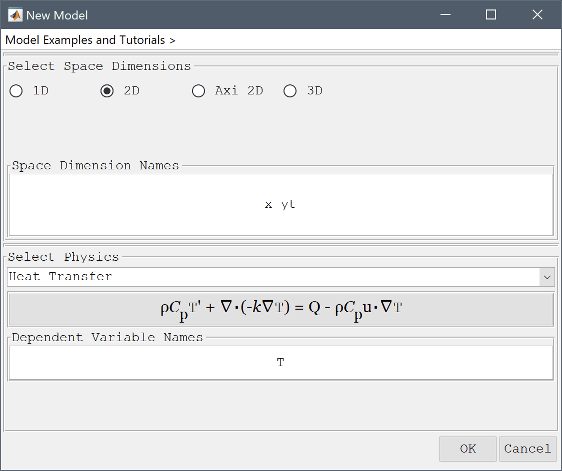
2. In the New Model dialog box, select 2D for the Space Dimensions, change the name of the space dimension coordinate names to x to represent the length dimension and yt to represent the time axis (t is a reserved variable name for time/test function and should not be used), and select Heat Transfer from the Select Physics drop-down menu. Leave the dependent variable name to the default and press OK to finish the physics mode selection.

   
3. Press OK to finish the physics mode selection.

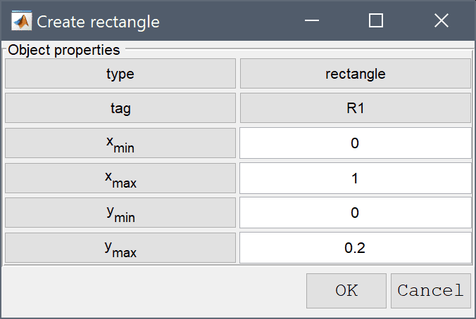
The original problem examines a 1 m rod during 0.2 s, so the equivalent 2D geometry is a rectangle spanning 0 x 1 and 0 x 0.2 where the y-direction will represent the time axis.

1. Select Rectangle from the Geometry menu.
2. Enter 0 into the x_min edit field.
3. Enter 1 into the x_max edit field.
4. Enter 0 into the y_min edit field.

5. Enter 0.2 into the y_max edit field.

   
6. Press OK to finish and close the dialog box.
7. Switch to Grid mode by clicking on the corresponding Mode Toolbar button.
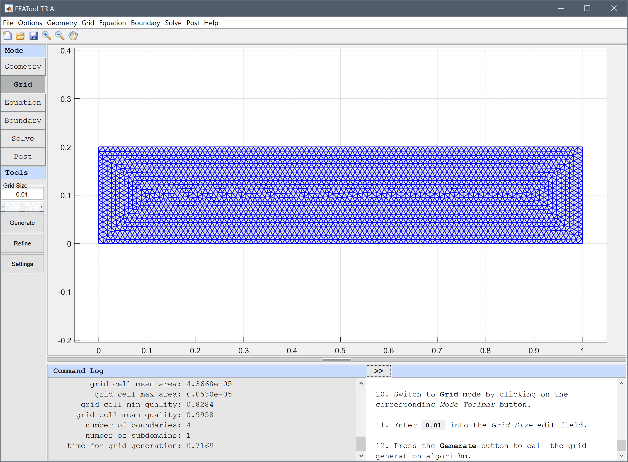
8. Enter 0.01 into the Grid Size edit field.

9. Press the Generate button to call the grid generation algorithm.

   
10. Switch to Equation mode by clicking on the corresponding Mode Toolbar button.

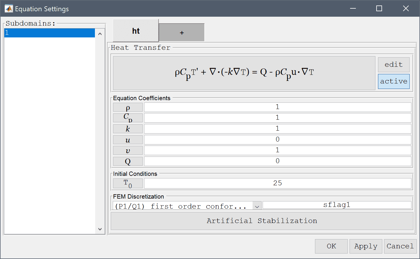
The density, heat capacity, and thermal conductivity are all assumed equal to one.

1. Enter 1 into the Density edit field.
2. Enter 1 into the Heat capacity edit field.
3. Enter 1 into the Thermal conductivity edit field.

Although the problem doesn't involve any convection, the resulting time discretization term is here represented by a convective term in the positive y-direction (time flowing from y = 0 upwards).

1. Enter 0 into the Convection velocity in x-direction edit field.
2. Enter 1 into the Convection velocity in yt-direction edit field.
3. Enter 0 into the Heat source edit field.

4. Enter 25 into the Initial condition for T edit field.

   
5. Press the edit button.

The modified equation must be changed to remove the thermal conduction term from the time axis (y-direction).

1. Enter -k_ht*Tx_x + rho_ht*cp_ht*u_ht*Tx_t + rho_ht*cp_ht*v_ht*Tyt_t = q_ht into the Equation for T edit field.

   
2. Press OK to finish and close the dialog box.
3. Press OK to finish the equation and subdomain settings specification.
4. Switch to Boundary mode by clicking on the corresponding Mode Toolbar button.

In the original one-dimensional the initial temperature is a constant 25 degrees, in the transformed problem this is equivalent to prescribing a constant temperature at the bottom boundary.

1. Select 1 in the Boundaries list box.
2. Select Temperature from the Heat Transfer drop-down menu.

The left and right boundaries are prescribed fixed temperature and heat flux conditions just as in the original problem.

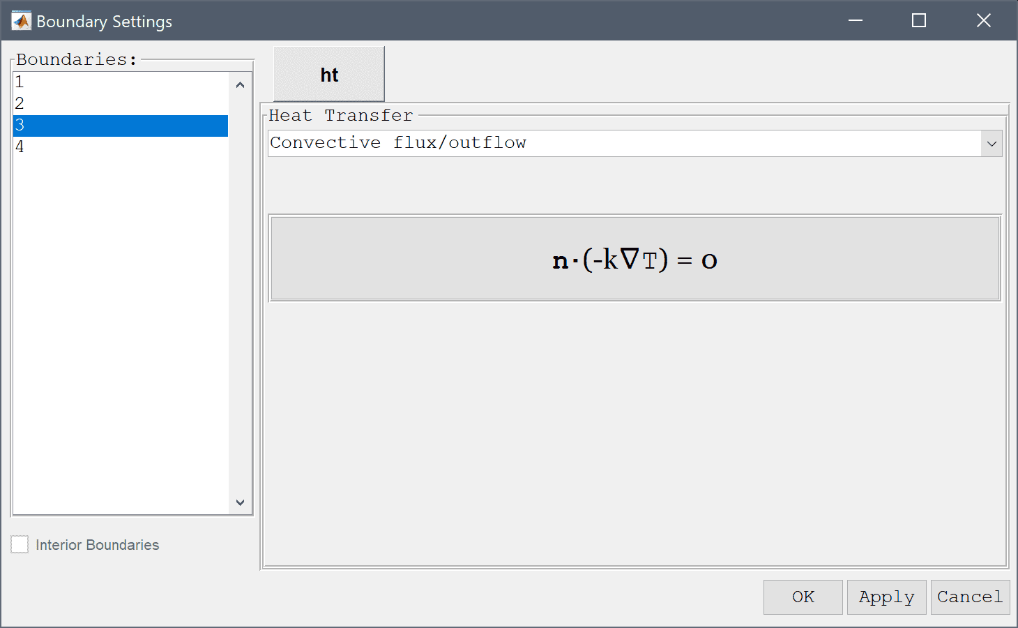
1. Enter 25 into the Temperature edit field.
2. Select 2 in the Boundaries list box.
3. Select Temperature from the Heat Transfer drop-down menu.
4. Enter 25 into the Temperature edit field.
5. Select 4 in the Boundaries list box.
6. Select Heat flux from the Heat Transfer drop-down menu.
7. Enter -1 into the Inward heat flux edit field.

Lastly, the top boundary where time unknown is represented by a free/or convective outflow boundary condition.

1. Select 3 in the Boundaries list box.

2. Select Convective flux/outflow from the Heat Transfer drop-down menu.

   
3. Press OK to finish the boundary condition specification.
4. Switch to Solve mode by clicking on the corresponding Mode Toolbar button.
5. Press the = Toolbar button to call the solver. After the problem has been solved FEATool will automatically switch to postprocessing mode and plot the computed solution.
6. Press the Plot Options Toolbar button.
7. Select the Enable/disable contour plot check box.

8. Press OK to plot and visualize the selected postprocessing options.

   

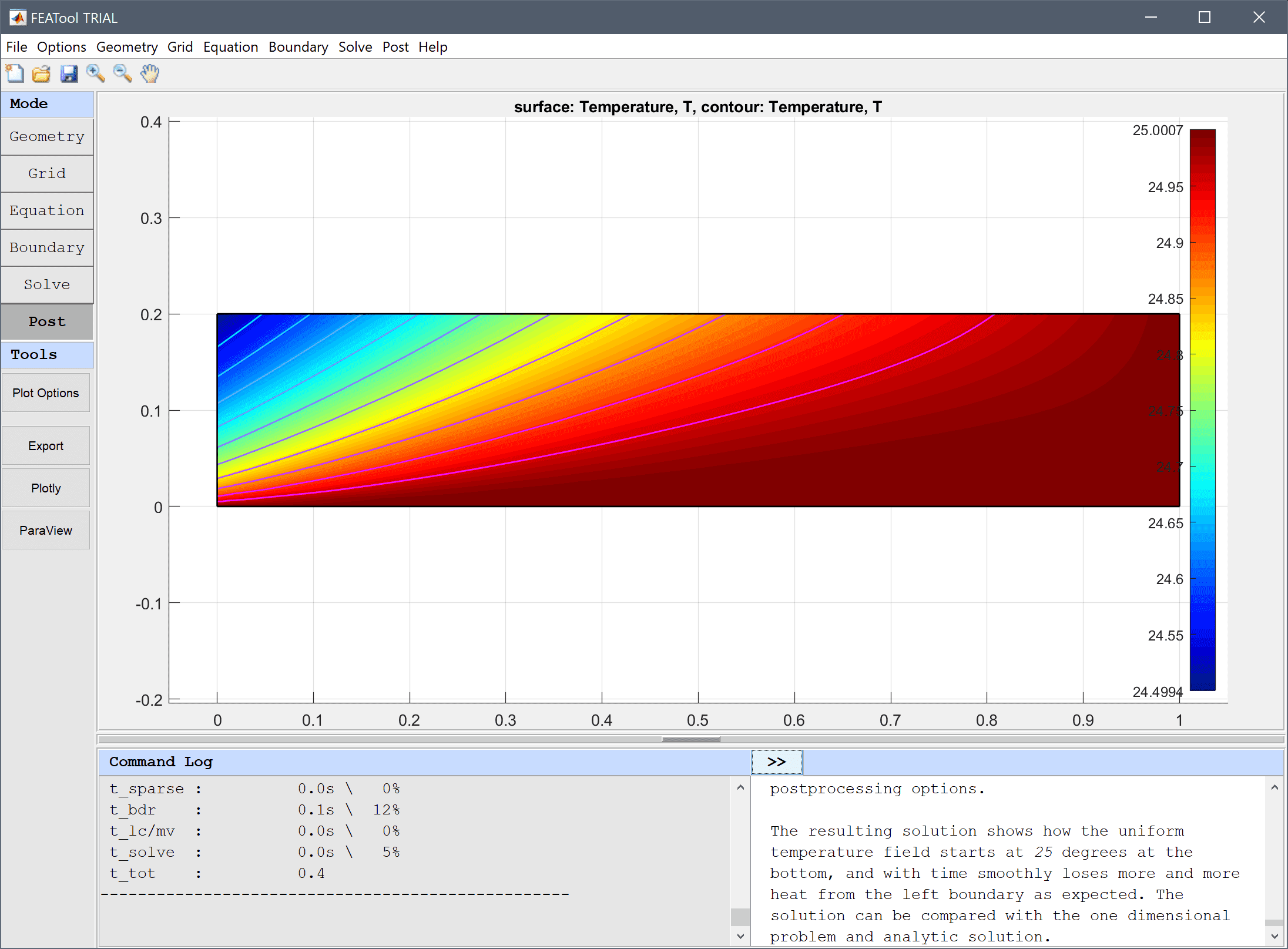
The resulting solution shows how the uniform temperature field starts at 25 degrees at the bottom, and with time smoothly loses more and more heat from the left boundary as expected. The solution can be compared with the one dimensional problem and analytic solution.

The space-time transformation of heat conduction heat transfer model has now been completed and can be saved as a binary (.fea) model file, or exported as a programmable MATLAB m-script text file (available as the example ex_heattransfer8 script file), or GUI script (.fes) file.