|
|
FEATool Multiphysics
v1.18.0
Finite Element Analysis Toolbox
|
|
|
FEATool Multiphysics
v1.18.0
Finite Element Analysis Toolbox
|
The first step in the modeling process is to create a geometry which defines the domain to be simulated. The geometry is used by the grid generation algorithm to compute a corresponding mesh on which the simulations are performed.
This section describes how geometries can be created in FEATool Multiphysics either by combining geometry primitives such as rectangles, circles, blocks, and cylinders etc. or importing existing geometry designs from CAD (Computer-Aided Design) format files.
Geometry mode is the default processing mode that new models start in. This mode can also be selected by pressing the ![]() mode button or by choosing the corresponding menu item labeled Geometry Mode. While in geometry mode the Tools toolbar will contain buttons that represent the geometry objects that can be created as well as the available geometry operations.
mode button or by choosing the corresponding menu item labeled Geometry Mode. While in geometry mode the Tools toolbar will contain buttons that represent the geometry objects that can be created as well as the available geometry operations.
A geometry object Selection list box is also be available in geometry mode, (either directly below the geometry Tools frame or in its separate figure window if not enough space is available), which can be used to select geometry objects to perform and apply operations on. In three dimensions (3D), individual faces of geometry objects can also be selected for the chamfer, extrude, fillet, loft, revolve and workplane operations. (The list of 3D faces is expanded when the corresponding object is double clicked on in the selection list box.)
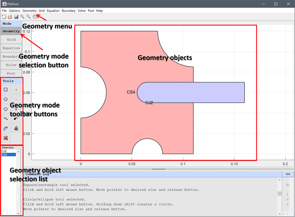
Geometry objects can also be selected by (left) clicking on them with the mouse cursor in the plot axes of the main GUI window (when no other visualization tools are selected such as pan, zoom, and rotate). In 3D, Ctrl+click also allows for mouse selection/de-selection of individual faces. The keyboard shortcuts Ctrl+A selects all geometry objects, while Ctrl+D de-selects them. The main plot axes will show all present geometry objects and highlight them in red color when they are selected.
In two dimensions rectangles, squares, ellipses, circles, polygons, and NACA wing profile geometry object primitives are available. To create a two-dimensional geometry object click on one of the corresponding toolbar buttons
In three dimensions solid block, cone, cylinder, ellipsoid, polyhedron, sphere, and torus geometry object primitives are available. To create a 3D geometry object click on one of the corresponding toolbar buttons
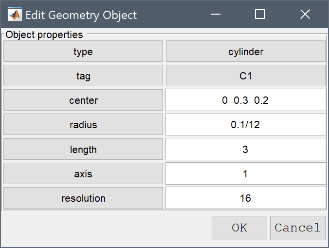
This will open a dialog box where the dimensions of the corresponding objects and properties can be entered
The Create Object... option in the Geometry menu also allows for the geometry objects described above, as well as point objects which are used to enforce grid vertices at the specified points during the grid generation process.
Pressing the Inspect/edit selected geometry object ![]() button will open a dialog box for the selected geometry object where object properties can be edited.
button will open a dialog box for the selected geometry object where object properties can be edited.
Subdomains are defined by either touching but non-intersecting, or completely disconnected geometry objects. Different subdomains can be used to define separate parameters and equation coefficients in different material regions of the model (see for example the heat transfer model Shrink Fitting of an Assembly). One can also deactivate equations in different parts so that different physics modes are active in different regions (see for example the Flow in Porous Media tutorial model).
If more than one geometry object is present in the final geometry the geometry algorithm will split it along all overlapping regions and intersecting boundaries before grid generation. This creates subdomains of the decomposed minimal regions, as in the illustration below.
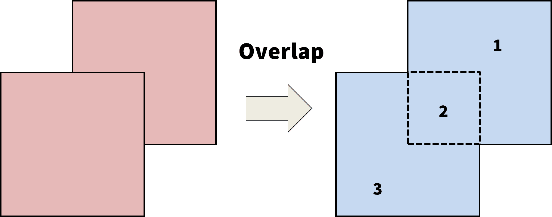
Interaction between subdomains occur at inner or internal boundaries, which by default are prescribed with continuity conditions (homogeneous Neumann). To access boundary specification on inner boundaries, at least one physics mode in a subdomain needs to be deactivated (as this computes the internal boundaries, but can later be activated again). The normal for flux boundary conditions on inner boundaries is defined to point from the subdomain with higher number to lower.
Geometry operations can be used to transform geometry objects and build more complex shapes from the primitives. The available operations are described in the following, and can be applied to selected objects by either using the corresponding buttons in the Tools toolbar or menu items in the Geometry menu.
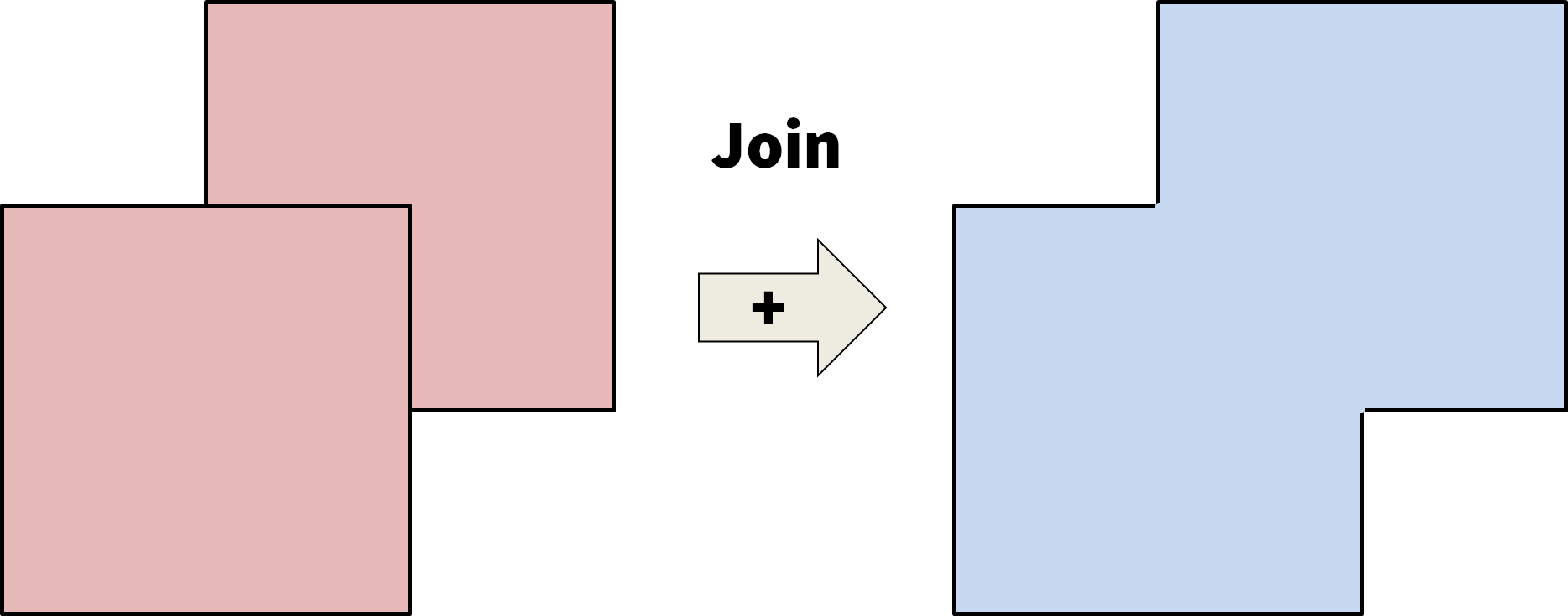
The Constructive Solid Geometry (CSG) operations, join, intersect, and subtract, allow intersecting/touching geometry objects to be combined to form more complex geometries and shapes.
The join operation (also commonly called union or fuse) merges all selected geometry objects to a single composite object. Select two or more objects to merge and then press the join ![]() button. Embedded boundaries and faces will in general not be removed but kept in the resulting object (for example joining two unit cubes result in a 1 by 2 block with 10 instead of 6 boundaries).
button. Embedded boundaries and faces will in general not be removed but kept in the resulting object (for example joining two unit cubes result in a 1 by 2 block with 10 instead of 6 boundaries).
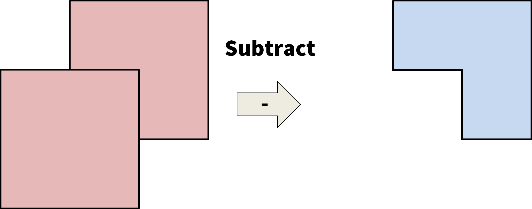
The subtract (difference / cut) ![]() operation removes overlapping regions from the largest of the selected geometry objects. Note that two or more resulting objects may be created if the cutting object(s) completely splits the object to cut.
operation removes overlapping regions from the largest of the selected geometry objects. Note that two or more resulting objects may be created if the cutting object(s) completely splits the object to cut.
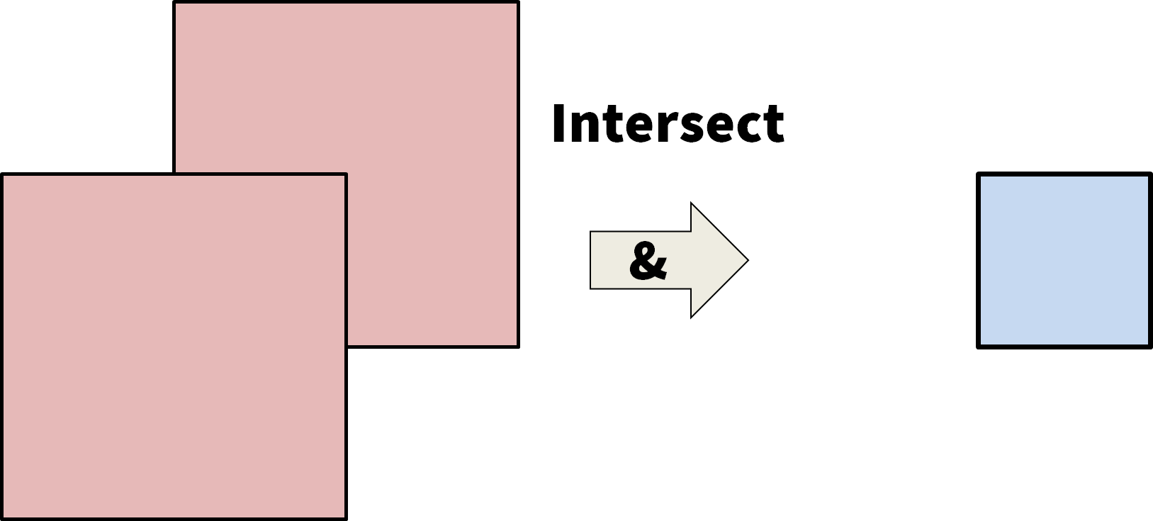
The intersect (common) ![]() operation returns the intersection or overlapping region of all of the selected geometry objects.
operation returns the intersection or overlapping region of all of the selected geometry objects.
For precise control of CSG geometry operations, one can select and use the Combine Objects... option in the Geometry menu, which opens a dialog box where an exact geometry formula can be entered. The syntax uses + for join, - for subtract, and & for the intersection operation as well as the geometry object labels or tags shown in the geometry object Selection listbox. The CSG operations are generally applied from left to right according to the given formula. (Take care that CSG operations only can be used on objects that touch or intersect.)
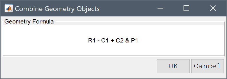
In the example here R1 - C1 + C2 & P1, circle C1 will first be subtracted from rectangle R1. The intermediate result will be joined with C2, after which it will be intersected with the polygon object P1.
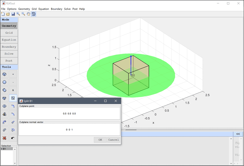
The split operation allows splitting geometry object(s) by a line in 2D or plane in 3D. After selecting object(s) to split and pressing the corresponding split ![]() button, a dialog box will open where one can define the splitting line or plane (by point and cutline direction/cutplane normal vectors). The splitting line/plane is also visualized in the main plot axes.
button, a dialog box will open where one can define the splitting line or plane (by point and cutline direction/cutplane normal vectors). The splitting line/plane is also visualized in the main plot axes.
Transformation operations allows one to move (linear translation), scale, and rotate geometry objects, in addition to producing copies. Selecting the copy and/or transform object ![]() button opens a dialog box where one can prescribe the desired transformations.
button opens a dialog box where one can prescribe the desired transformations.
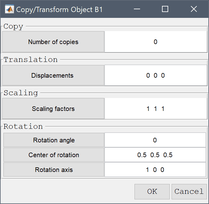
The copy operation allows making a number of copies of selected objects. If any of the transformation operations are non-zero they will also be performed in the sequence move, scale, and rotate for each copy. The transformations when copying are applied additively so that for example a prescribed move/translation will be applied n times for the n:th copy.
Linear translation/movement is specified as a space separated vector of a translation distance or displacement length in each space dimension/direction (can be negative). All entries are set to zero by default (no translation).
The scale operation is specified as a non-zero space separated vector for the scaling factor in each space dimension/direction (a negative value will mirror the object in the corresponding direction). All scaling entries are set to one by default (no scaling).
The rotation operation allows prescribing a rotation around a point or axis. In 2D, rotation is described by a rotation angle (in degrees) and a point (indicating counter-clockwise rotation for a positive angle around the specified point). In 3D, rotation is specified with an angle (in degrees) and axis around which the rotation should occur (with positive angle indicating rotation according to the right hand rule with respect to the axis). The rotation angle is zero by default (no rotation).
The chamfer operation is used to apply straight bevels to vertices in 2D and edges in 3D. To apply chamfers, first select the desired object(s), and then press the corresponding chamfer ![]() tool button. A dialog box will open where one can further select the vertices/edges to chamfer, and the desired chamfer distance.
tool button. A dialog box will open where one can further select the vertices/edges to chamfer, and the desired chamfer distance.
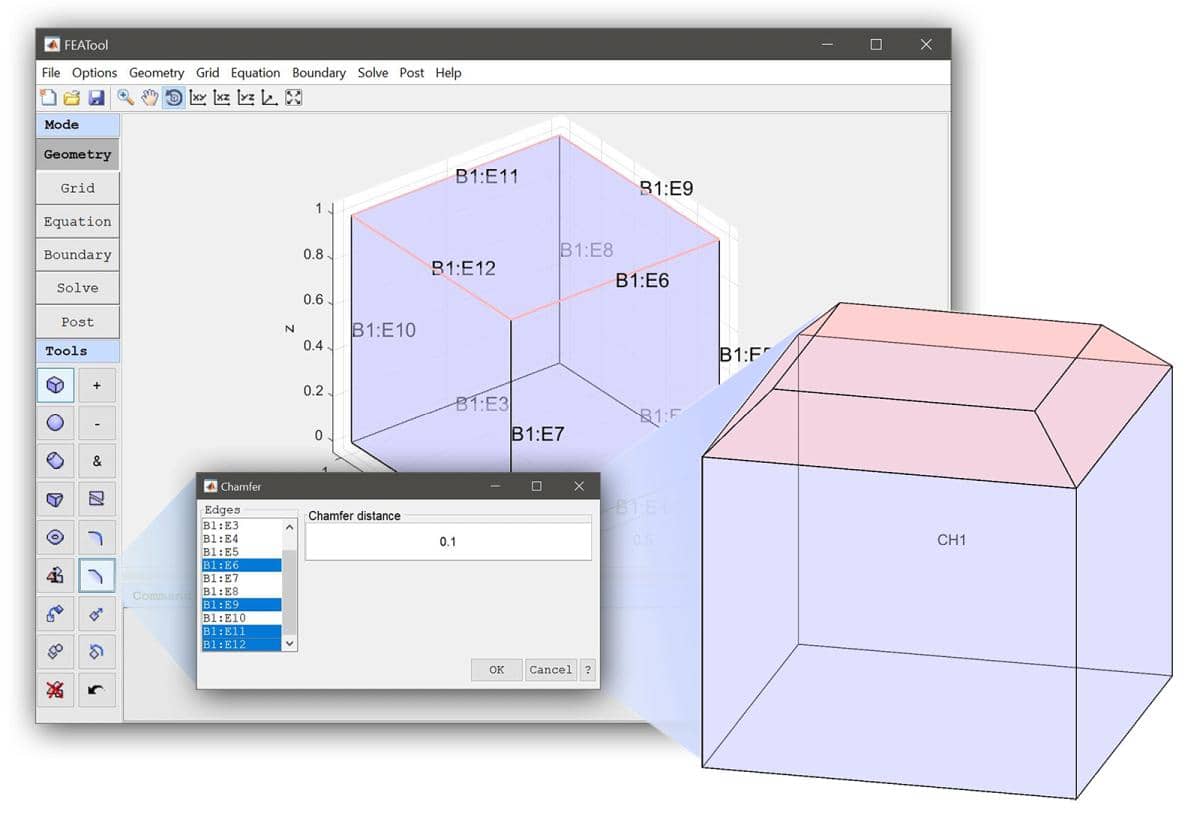
Note that the construction of chamfers can be algorithmically difficult and the geometry engine may fail for complex cases, especially when the end point of a chamfer contour is the point of intersection of four or more edges of a shape, or the intersection of the chamfer/fillet with a face which limits the contour is not fully contained in this face. If a multi-select chamfer operation fails, it can help to apply operations one-by-one to vertices/edges.
The fillet (round) operation is used to apply rounded bevels to vertices in 2D and edges in 3D. To apply fillets, first select the desired object(s), and press the corresponding fillet ![]() tool button. A dialog box will open where one can further select the vertices/edges to fillet, the desired fillet radius.
tool button. A dialog box will open where one can further select the vertices/edges to fillet, the desired fillet radius.
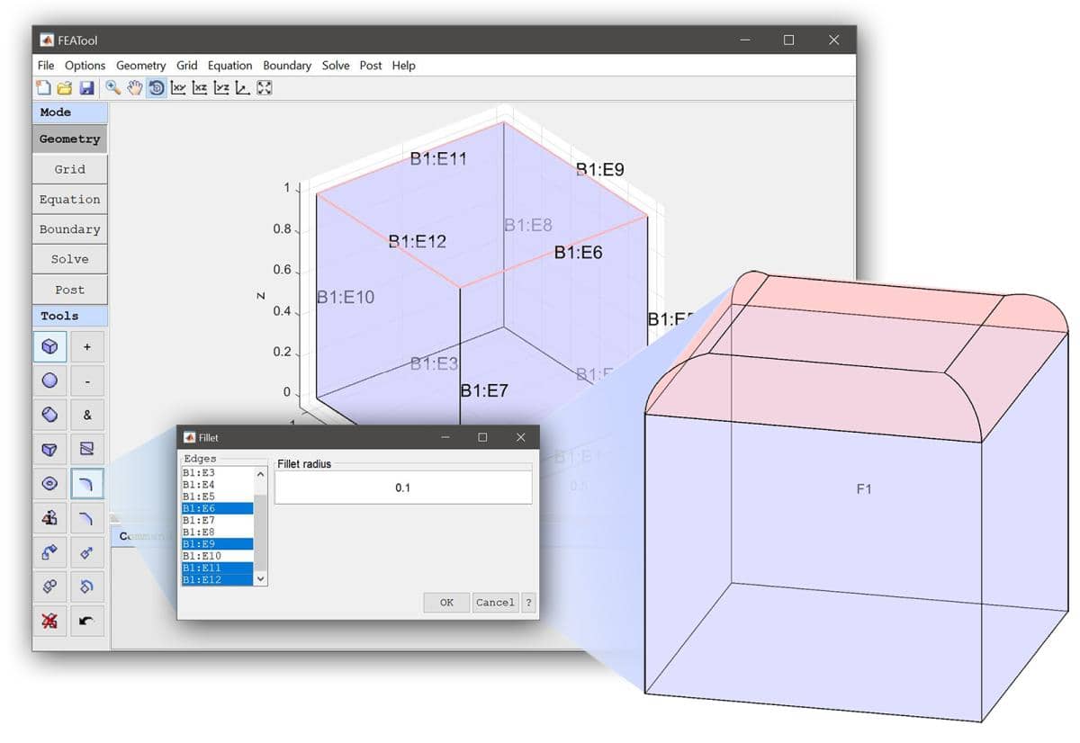
Note that the construction of fillets can be algorithmically difficult and the geometry engine may fail for complex cases, especially when the end point of a fillet contour is the point of intersection of four or more edges of a shape, or the intersection of the chamfer/fillet with a face which limits the contour is not fully contained in this face. If a multi-select fillet operation fails, it can help to apply operations one-by-one to vertices/edges.
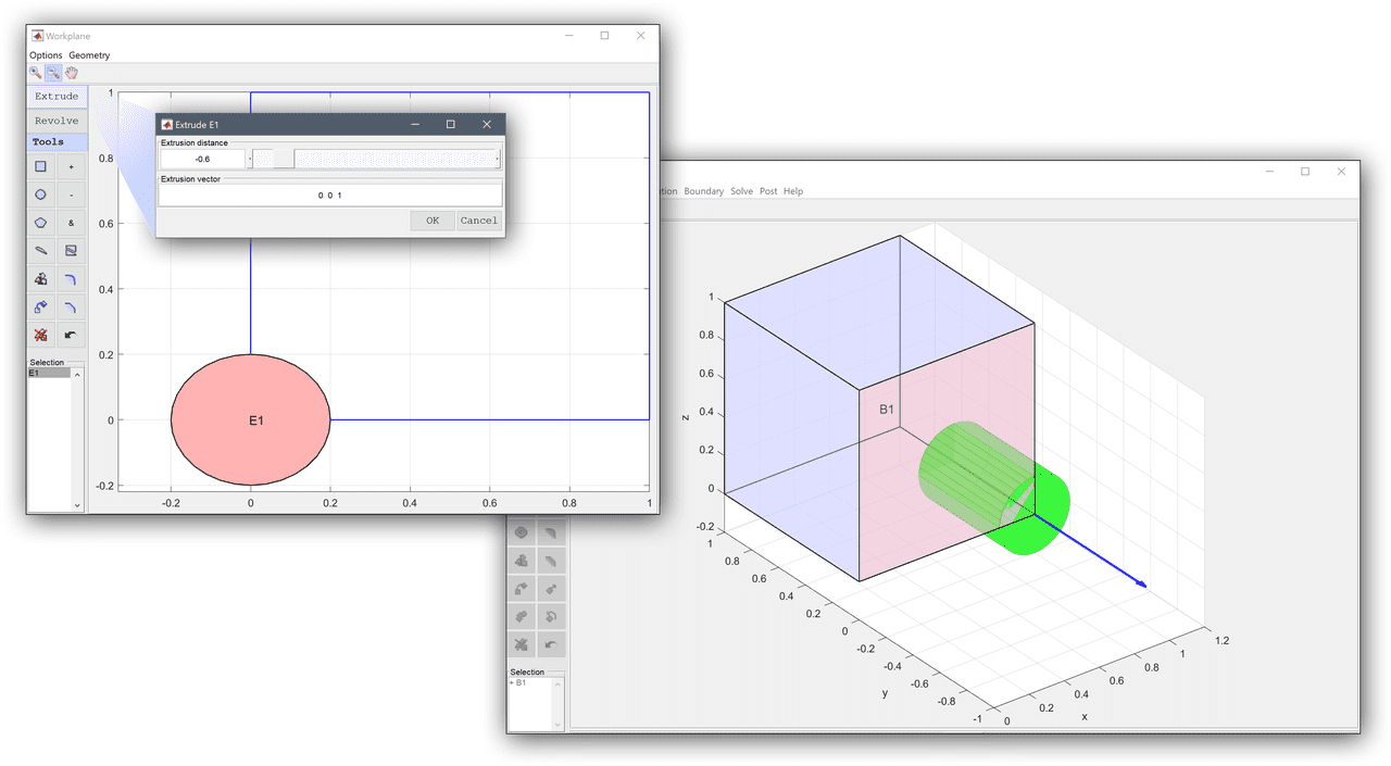
The extrude operation allows a selected face from a 3D object to be extruded in a direction to a solid shape. To make an extrusion object first select the face to extrude, and then press the extrude ![]() button. The extrude dialog box will open where both the extrusion distance and direction vector can be specified. A preview of the extrusion object with selected parameters can be seen highlighted in green in the main plot axes with a blue arrow indicating the direction of the extrusion.
button. The extrude dialog box will open where both the extrusion distance and direction vector can be specified. A preview of the extrusion object with selected parameters can be seen highlighted in green in the main plot axes with a blue arrow indicating the direction of the extrusion.

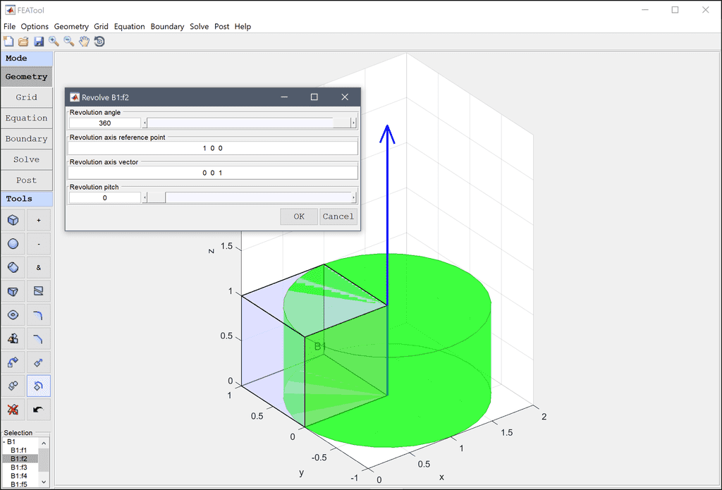
The revolve operation allows a selected face from a 3D object to be revolved around an axis to a solid shape. To make a revolution object first select the face to revolve, and then press the revolve ![]() button. The revolve dialog box will open where both the revolution angle (degrees), axis reference point and vector can be specified. A revolution object can also be given a pitch to create a coil (see for example the Stress Distribution in a Solenoid tutorial model). A preview of the revolution object with selected parameters can also be seen highlighted in green in the main plot axes.
button. The revolve dialog box will open where both the revolution angle (degrees), axis reference point and vector can be specified. A revolution object can also be given a pitch to create a coil (see for example the Stress Distribution in a Solenoid tutorial model). A preview of the revolution object with selected parameters can also be seen highlighted in green in the main plot axes.
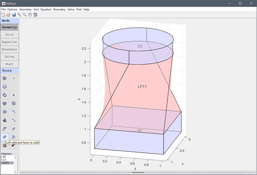
The loft operation allows creation of a swept solid object with a smooth transition between several faces. To create a loft object first select two or more faces, and then press the loft ![]() button. (Note that faces to loft can not all be in the same plane with identical normal vectors.)
button. (Note that faces to loft can not all be in the same plane with identical normal vectors.)
The defeature operation can be used to clean up imported 3D CAD geometries by removing features such as small holes, thin chamfers, fillets, grooves, threads, and embedded text. Defeaturing can significantly simplify geometries, which makes meshing easier, and simulations more efficient and faster.
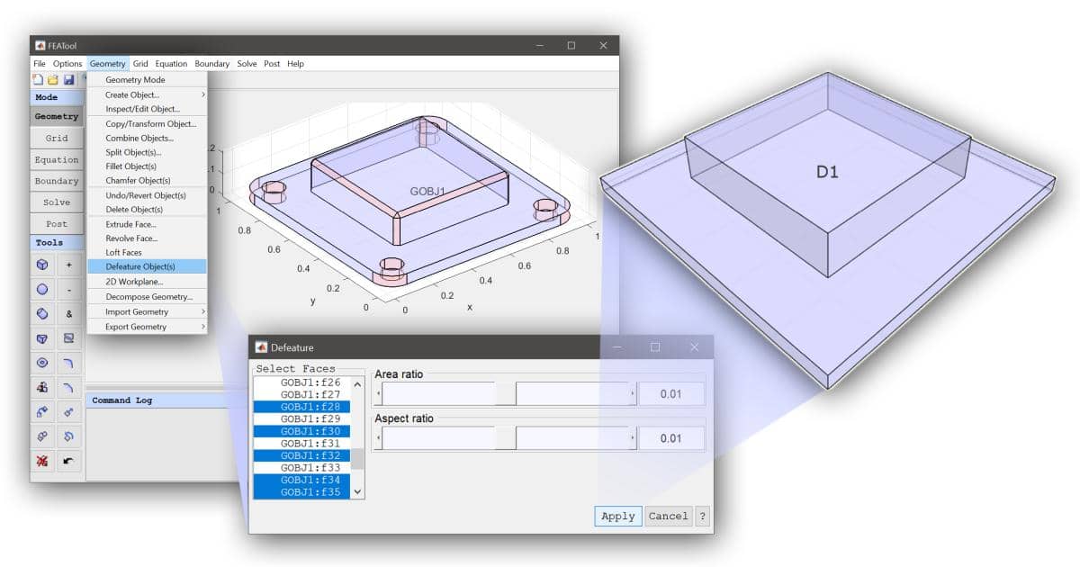
To use defeaturing, first select Defeature Object(s) from the Geometry menu. A dialog box will open. Select faces to try to remove in the left listbox, or hold the Ctrl key while clicking with the mouse on a face to select/de-select it. If for example on wishes to remove a hole, select all inner faces of the hole.
Alternatively, automatic face selection can also be performed by selecting the Area and Aspect ratio controls. The area ratio control selects faces with area to total object area smaller than the specified ratio (default 1%), thus detecting small faces. Similarly, the aspect ratio selects faces with ratio of shortest to longest boundary box edge below the given threshold (default 1%), detecting thin sliver faces.
Once faces have been selected, press Apply to perform the defeaturing operation. If the operation is successful a new simplified object will be returned without the selected faces. If the operation is not successful one can try reducing the number of faces to simplify in each defeaturing step.
By pressing the delete ![]() button the selected geometry object(s) will be completely deleted. (Note that the last deleted geometry object can be restored using the undo/revert button.)
button the selected geometry object(s) will be completely deleted. (Note that the last deleted geometry object can be restored using the undo/revert button.)
The undo/revert ![]() button is used to undo a previous join, subtract, intersect, split operation or transformation operations such as move, scale, rotate, chamfer, and fillet and returns the original input/parent objects. If no objects are selected the last deleted geometry object can also be restored if desired.
button is used to undo a previous join, subtract, intersect, split operation or transformation operations such as move, scale, rotate, chamfer, and fillet and returns the original input/parent objects. If no objects are selected the last deleted geometry object can also be restored if desired.
The Decompose Geometry... menu option allows for the geometry objects to be split into decomposed and non-overlapping objects/subdomains (this is performed automatically before grid generation). Note that the original geometry objects will be discarded but can be retrieved using the Undo operation (before any other objects have been discarded).
Three dimensional shapes can also be created with the help of sketching and drafting planar shapes on a 2D workplane, after which they can be extruded and revolved to solid shapes into the 3D space.
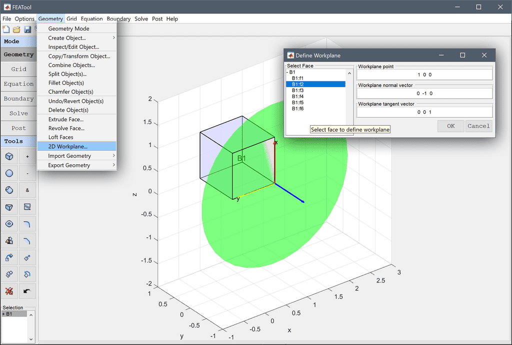
To create a workplane, first select 2D Workplane... from the Geometry menu. The Define Workplane dialog box will open where a point, and normal and tangent vectors can be specified to define the workplane. If any geometry objects are present a selection list box will also be available where one can select a face from which the workplane can be defined from. The workplane is visualized in the plot axes as a green circle with red, yellow, and blue arrows in the origin which represent and will define the x, y, and z-axis in the local coordinate system of the workplane.
A workplane starts a new GUI figure window with tools for 2D geometry creation. The outline of existing 3D objects projected onto the workplane plot axes will be shown in blue. After creating 2D shapes in the workplane, one can select either the ![]() or
or ![]() button to perform the corresponding operation into the 3D space. A preview of the resulting shape will be shown in the 3D GUI before confirming the operation. Control will be reverted to the original 3D window after closing and exiting the workplane GUI. The Stress Distribution in a Solenoid tutorial illustrates how to use a 2D workplane and revolve a sketch to a 3D shape.
button to perform the corresponding operation into the 3D space. A preview of the resulting shape will be shown in the 3D GUI before confirming the operation. Control will be reverted to the original 3D window after closing and exiting the workplane GUI. The Stress Distribution in a Solenoid tutorial illustrates how to use a 2D workplane and revolve a sketch to a 3D shape.
The examples in the tutorial sections include step-by-step guides how to create different types of geometries. For example, the Thin Plate with Hole model shows how to make a rectangle with a circular corner and Shrink Fitting of an Assembly describes how to create a complex assembly with several subdomains, the Stress Distribution in a Solenoid tutorial illustrates how to use a 2D workplane and revolve a sketch to a 3D shape, and the Deformation of a Spanner example shows how to import a pre-made geometry from a CAD file.
Import and export of CAD geometries is supported through the corresponding Import Geometry and Export Geometry menu options. Geometry import and export is supported for FEATool geometry BREP, IGES, OBJ, PLY, STL, and STEP CAD file formats, as well as Gmsh struct variables from the main MATLAB workspace, ASCII and binary (geo) and 2D Triangle (poly), and bitmap image formats (BMP, JPG, PNG, TIFF).
Care should be taken when preparing CAD models, as simulation and meshing requires very precise geometries. Although basic automatic CAD repair is built-in with the FEATool toolbox, it is recommended to prepare CAD files so that they are water tight, that is do not have disconnected holes, regions, or duplicated and overlapping facets and structures in them. It is also recommended to try to reduce the number of features and scale differences between them (as a large jump in scale between features may cause issues with meshing).
Import of BIN, BREP, IGES and STEP CAD geometries are supported through the corresponding menu options. In contrast to the STL format, the BREP, IGES and STEP formats contain boundary and surface feature information and are therefore the recommended CAD formats to use. Although, BIN/BREP/IGES/STEP geometries can be combined with other geometry objects or modified after import, it is recommended to have a finished geometry representation before importing. The Gmsh external mesh generator is also required to generate grid for these types of CAD geometries.
Mesh based geometry shape formats such as STL and Wavefront OBJ are supported for both geometry import and export. However, in contrast to CAD formats with boundary representation (BREP, IGES, and STEP), mesh based formats are not as exact in as they only represent the geometry shapes approximately (as a collection of mesh facets). Mesh based geometries should therefore only be used if other CAD formats are not available. (Note that converting a mesh to for example STEP format does not help, as a conversion cannot reconstruct the original shape.)
Both binary and ASCII Stereolithography file import is supported for both full 3D, and (planar) 2D geometries. An OBJ or STL file is considered planar if all coordinates of one of the axes are equal (typically the z-coordinates are set equal to zero). Note that 3D geometries can only be imported into 3D models, and 2D geometries into 2D models.
STL import and export supports multiple solid sections (limited to ASCII STL format) and STL input files. For 2D geometries each solid section is processed as a separate subdomain, while for 3D objects each solid section is per default processed as separate boundaries for the same solid. Multiple 3D subdomains can optionally be processed by using multiple input files (each 3D STL input file corresponds to its own subdomain, while solid sections correspond to the boundary faces).
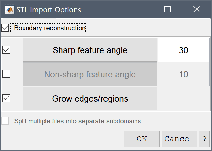
The STL Import Options dialog box (only available in 3D) allows control over automatic Boundary reconstruction and feature recognition, which tries to reconstruct and assign separate boundary surfaces from the imported STL facet data (default off). The Sharp feature angle specifies the maximum dihedral angle between facet edges to be considered a sharp feature edge. This is typically in the range 20-45 degrees, where a larger angle will detect more features. Non-sharp feature angle specifies the limit to define sharp needle, and flat cap triangles which can be used to detect in-plane features, that is features where a surface region changes structure. Grow edges/regions toggles whether loose edges without connections at the end points should be grown and extended to form closed surface patches (or eliminated). If multiple STL files have been given as input, the option to try to Split multiple files into separate subdomains will be available. Facets of shared boundaries between subdomains must in this case align without overlap for internal boundaries to be identified correctly.
An example utilizing CAD geometry import functionality is the Deformation of a Spanner tutorial which shows how to import a pre-made geometry from a CAD file. Manual command line interface CLI usage is also possible directly with the impexp_stl function allowing for fine tuning of import parameters. The mesh_analyze function can also be used manually to fine tune the detection of surface and boundary features.
CSG geometry operations (such as join, intersect, and difference) with mesh based geometry objects will first go through a conversion process. This can be very slow and inefficient if a geometry object consists of a large amount of facets (> 1000). In this case it is recommended to instead use the Robust mesh generation algorithm with the original faceted shapes as input directly and a CSG formula as Optional Parameter in the Grid Generation Settings (for example 'formula' 'OBJ1 - OBJ2'). So that the mesh generation algorithm will apply the CSG operation directly during meshing instead. Boundary reparametrization is by default off, but can be enabled using the Reparametrization Angle option, or performed as a manual reparametrization step after meshing.
If available boundary representation CAD formats (BIN, BREP, IGES, STEP) should always be used before the faceted formats (STL, OBJ, PLY). Moreover, conversion between faceted and boundary CAD formats is not recommended as in the conversion process significant boundary information is lost, which can not be recovered.
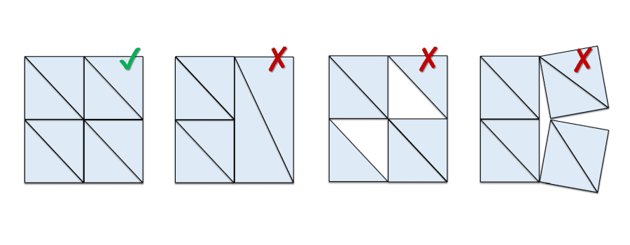
For 3D STL import best practice is to have the geometry pre-processed into separate boundaries and subdomains (by splitting the boundaries into solid sections and subdomains into files). It is also recommended that all facet edges are simply connected without overlaps. If the import process fails, try using CAD file repair in a dedicated external software prior to import. Correct and incorrect facet configurations is illustrated in the image below.
For STL geometries that can not be correctly imported due to poor quality of the mesh (typically generating a "could not match up all facet edges" error due to too large gaps between the facets in the STL file resulting in a non-watertight geometry), can be attempted to be imported and meshed as raw facet data with the boundary reconstruction option disabled. In this case no boundary reconstruction is attempted and the raw STL data will be passed directly to the grid generator for meshing and boundary reconstruction.
In general, for meshing difficult and faceted geometries it is recommended to use the Robust 3D grid generation option, which feature an angle parameter used to identify and separate facets in to boundaries (post meshing).
2D planar polygonal geometry objects can also be reconstructed from bitmap images (JPG, PNG, BMP, TIFF). Selecting Import Geometry > From Image... from the Geometry menu, first opens dialog box to select an image file. Once selected and loaded the following dialog box will open.
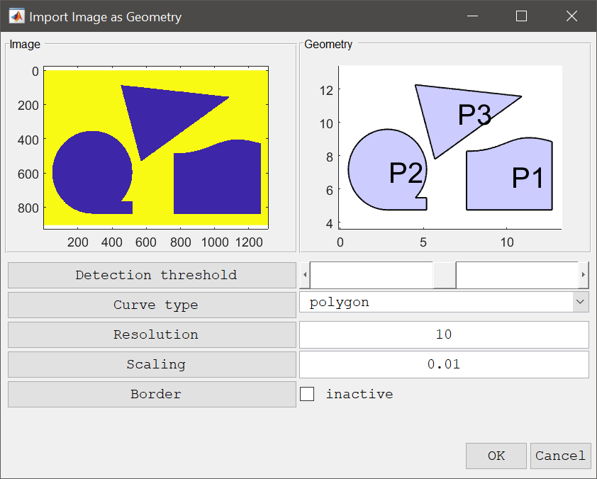
The left image shows the outlines of any detected objects, and on the right shows the reconstructed geometry objects.
The following controls allow modification and update of the image reconstruction. The Curve type selection listbox allows for switching between polygon (straight line), spline, and Bezier geometry object curve types. The Detection threshold slider can be used to adjust the threshold level for which to detect object edges. Resolution sets the number of pixels to use when reconstructing polygonal line segments (defaults to 10 segments per polygon shape). Scaling prescribes the scaling factor geometry unit length per pixel. Lastly, the Border flag can be used to add an inverted border around the image to also capture objects touching the border. (Press Enter after changing the controls to update the reconstructed objects if its not automatically performed.)
Note, that the 3D geometry engine is sometimes not quite robust enough to handle all cases of overlapping boundary faces. Thus it is recommended when subtracting objects to allow for this by creating subtraction objects larger than the desired domain (so that non parallel planes are avoided). For faster and more robust 3D geometry operations it is recommended to use an external and dedicated CAD software (such as for example Fusion 360 or FreeCAD) and import the CAD geometries in BREP, STEP, or IGES formats.
The following functions can be used on the command line to programmatically generate and modify objects and geometries. As you build your geometry in the FEATool GUI the steps to programmatically generate the geometry is also recorded and can be exported to a m-file script by selecting Save As MATLAB Script... from the File menu.
| Function | Description |
|---|---|
| copy_geometry_object | Create copy of geometry object |
| geom_add_gobj | Add geometry object to geom or fea struct |
| geom_analyze | Analyze and decompose geometry |
| geom_apply_chamfer | Apply chamfers to geometry object edges |
| geom_apply_fillet | Apply fillets to geometry object edges |
| geom_apply_formula | Apply formula to geometry objects |
| geom_apply_transformation | Apply transformation to geometry objects |
| geom_defeature | Remove/simplify selected faces from geometry object |
| gobj_extrude | Extrude a geometry object/face |
| geom_extrude_face | Extrude a face to a 3D solid object |
| geom_loft_faces | Create lofted solid between selected faces |
| geom_revert_object | Revert/undo geometry object operations |
| gobj_revolve | Revolve a geometry object/face |
| geom_revolve_face | Revolve a face to a 3D solid object |
| geom_split_object | Split geometry object by cutplane/cutline |
| geom_clean | Clean and compact geometry objects |
| gobj_boundaries | Recompute boundaries field of geometry object |
| geom2geo | Export geom struct to Gmsh GEO file |
| geo2geom | Import Gmsh GEO file to geom struct |
| gobj_block | Create a 3D block |
| gobj_circle | Create a circle in 2D |
| gobj_cone | Create a (truncated) cone in 3D |
| gobj_curve | Create a Bezier curve in 2D |
| gobj_cylinder | Create a cylinder in 3D |
| gobj_ellipse | Create an ellipse in 2D |
| gobj_ellipsoid | Create an ellipsoid in 3D |
| gobj_line | Create a 1D line |
| gobj_naca | Create a NACA 4-series wing profile |
| gobj_point | Create a point |
| gobj_polygon | Create a 2D polygon |
| gobj_polyhedron | Create a 3D polyhedron |
| gobj_rectangle | Create a 2D rectangle |
| gobj_sphere | Create a 3D sphere |
| gobj_spline | Create a spline curve in 2D |
| gobj_torus | Create a 3D torus |
| gobj_info | Show geometry object information |
| impexp_cad | BIN/BREP/IGES/STEP CAD geometry import and export |
| impexp_obj | OBJ CAD geometry import and export |
| impexp_stl | STL CAD geometry import and export |
| import_img | Import geometry from bitmap image |
| export_ply | PLY geometry export |
| mesh_analyze | Surface mesh feature detection |
| mesh_repair | Surface mesh repair |
| plotgeom | Plot and visualize geometry |