|
|
FEATool Multiphysics
v1.18.0
Finite Element Analysis Toolbox
|
|
|
FEATool Multiphysics
v1.18.0
Finite Element Analysis Toolbox
|
In Equation mode partial differential equations (PDEs) together with equation coefficients must be chosen to accurately describe the physical phenomena to be simulated. Furthermore, in Boundary mode suitable boundary conditions must be prescribed in order to account for how the model interacts with its surroundings (outside of the modeled geometry and grid).
After creating a suitable geometry and grid one can switch between equation and boundary modes by using the ![]() and
and ![]() mode buttons. The corresponding Equation and Boundary Settings dialog boxes will also automatically open. Each boundary and equation setting tab corresponds to a different physics mode present in the model and allow for specifying the equation and boundary coefficients, initial conditions, and finite element shape functions. The coefficients and boundary coefficients will vary depending on the chosen physics mode and are explained in the following sections. The equation settings also allow for different equation and initial conditions to be set on a per subdomain basis by selecting the subdomains in the left hand side Subdomain listbox.
mode buttons. The corresponding Equation and Boundary Settings dialog boxes will also automatically open. Each boundary and equation setting tab corresponds to a different physics mode present in the model and allow for specifying the equation and boundary coefficients, initial conditions, and finite element shape functions. The coefficients and boundary coefficients will vary depending on the chosen physics mode and are explained in the following sections. The equation settings also allow for different equation and initial conditions to be set on a per subdomain basis by selecting the subdomains in the left hand side Subdomain listbox.
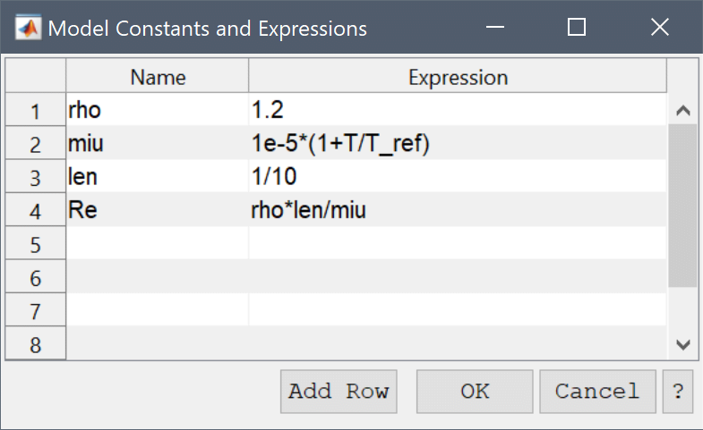
A convenient way to set up models is to use Model Constants and Expressions. The
Point ![]() (and 3D edge
(and 3D edge ![]() ) constraints are used to prescribe and precisely fix values on points (and edges), and is a Dirichlet type of boundary condition. When selected, the Point/Edge Constraints dialog box will show a table of point (or edge) numbers (rows), with corresponding dependent variables (columns). For point constraints, the available point locations can be selected among the vertices of the geometry and any point present objects. Constraints are specified by entering a non-empty value in the corresponding cell.
) constraints are used to prescribe and precisely fix values on points (and edges), and is a Dirichlet type of boundary condition. When selected, the Point/Edge Constraints dialog box will show a table of point (or edge) numbers (rows), with corresponding dependent variables (columns). For point constraints, the available point locations can be selected among the vertices of the geometry and any point present objects. Constraints are specified by entering a non-empty value in the corresponding cell.
Point sources ![]() can be used to prescribe source terms on specific points. In contrast to point constraints which prescribes fixed values, point sources impose loads/forces on specific points.
can be used to prescribe source terms on specific points. In contrast to point constraints which prescribes fixed values, point sources impose loads/forces on specific points.
Integral constrains ![]() are available to be set on both subdomains and also boundaries. This constraint type enforces the integral (sum) of a solution variable to be a prescribed value (such as for example enforcing a mean pressure over a domain or boundary).
are available to be set on both subdomains and also boundaries. This constraint type enforces the integral (sum) of a solution variable to be a prescribed value (such as for example enforcing a mean pressure over a domain or boundary).
The FEATool GUI also makes it easy to add and couple multiphysics equations and complex expressions to your models.
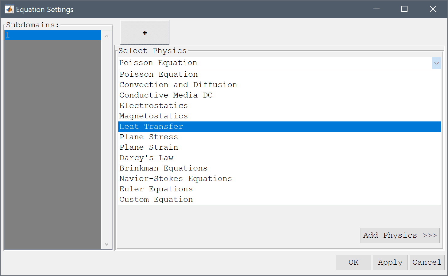
After starting to work with a physics mode it is simple to add one or more other modes by going to the last tab, with a + plus sign, in the Equation Settings dialog box. There you can simply choose an additional physics mode from the drop down combo box, select the dependent variable names you want to use (or keep the default ones), and press Add Physics >>> to add the mode. The new physics mode will now show up as a new tab with its short abbreviated name on the tab handle. Once the new mode has been added you can switch between the modes by clicking on the corresponding tabs in the Equation and Boundary Settings dialog boxes.
The physics modes can be coupled by simply using the dependent variable names and derivatives in the coefficient expression dialog boxes. For example, the Navier-Stokes equations physics mode shown below uses the temperature variable T from the heat transfer mode in the source term for the y-direction.

Moreover, here below we can see how to make a three way multiphysics coupling. The convective velocities u and v are coupled from the Navier-Stokes equations physics mode and at the same time the temperature T and its two derivatives Tx and Ty are simultaneously coupled to the reaction rate source term in the convection and diffusion mode.
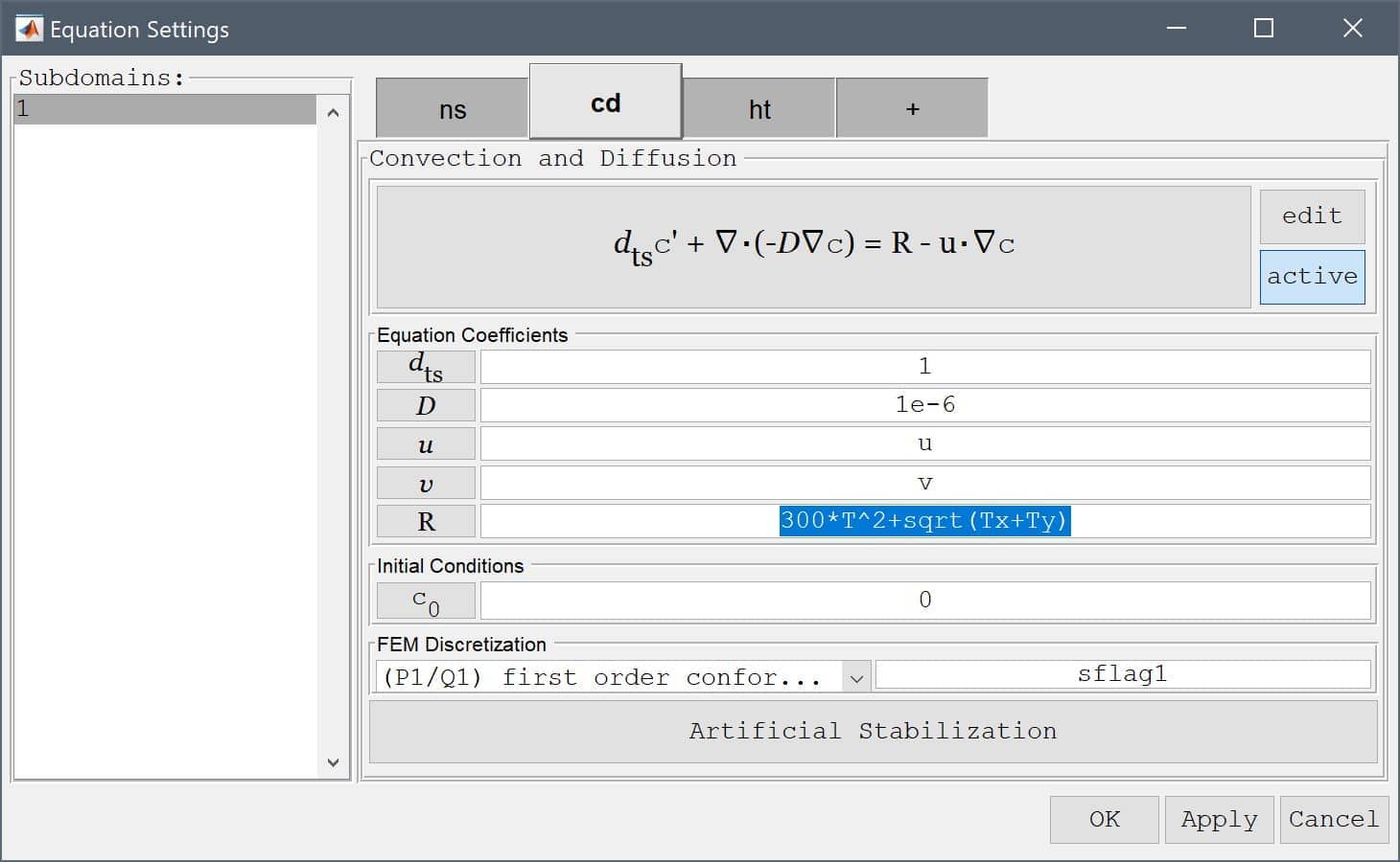
As we have seen, it is very simple to set up multiphysics models in FEATool. This is made possible by the expression parsing functionality that allows you to enter and use complex expressions of dependent variables (for example u, v, T, c), their first derivatives (by just appending x or y to the variable names like Tx and Ty), the space dimensions x and y, as well as all common MATLAB expressions and constants like pi, sin, cos, sqrt, ^2 etc.
FEATool Multiphysics conveniently features built-in parsing and evaluation of non-constant variables and coefficients This allows users to quickly and easily enter modeling expressions formulated much as one would write on paper, all without having to develop, write, and compile external user defined functions as other more complex simulation software often requires.
The following applies to all physics coefficients such as point constraints, boundary conditions, equation coefficients, initial conditions and postprocessing expressions, as well as command line functions such as evalexpr, intsubd, intbdr, minmaxsubd, minmaxbdr, and postplot. A coefficient may be composed as a string expression including any number of the various coefficient types listed below, combined with the operators +-*/^, parentheses pairs (), as well as numeric constants and scalars.
The space coordinates x, y, and z for Cartesian coordinate systems, and r and z for axi-symmetric and cylindrical coordinate systems are valid coefficient expressions. (Note that the space coordinate names can be re-assigned from their default definitions when starting a New Model).
The y-coordinate is for example used to define a parabolic velocity inlet profile as uinlet = 4*0.3/0.41^2*y*(0.41-y) in the flow around a cylinder CFD tutorial example.
Solution unknowns or dependent variables can also be used in coefficients, with their corresponding names given by the included physics modes, such as for example T for temperature. (As with the space coordinate names, dependent variable names may also be re-defined from the default names when a new physics mode is added. Also note that adding dependent variables in coefficients often make a problem more non-linear and harder to solve.)
The introductory heat transfer multiphysics model for example shows how the temperature T is coupled to the fluid flow via the source term alpha*g*rho*(T-Tc), where alpha, g, rho, and Tc, are model constants, while the flow velocities u and v in turn are coupled back and driving the temperature field through the convective terms.
By appending a space coordinate postfix to a dependent variable, for example Tx, the derivatives in the corresponding direction can be evaluated (in the example here Tx is equivalent to ∂T\∂x. The capacitance in the spherical capacitor model tutorial is for example calculated by integrating the expression eps0*epsr*(Vr^2+Vz^2)*pi*r, where V is the computed potential.
Second order derivatives, as for example Txy equivalent to ∂2T\∂x∂y, can also be evaluated for dependent variables discretized by the second order Lagrange finite element basis functions.
Note that derivatives of dependent variables are evaluated by direct differentiation of the underlying FEM shape function polynomials and some overall accuracy may be lost in this process. For example, a variable discretized with a first order linear basis function, will feature a piecewise constant first derivative on each element, and zero second derivative (even if a global second derivative would exist analytically). For higher order accuracy with derivatives a projection or gradient reconstruction technique is necessary.
The variable name t is reserved for the current time in instationary simulations (evaluates to 0 for stationary problems). For example, the instationary flow around a cylinder example defines a parabolic and time dependent inlet velocity as uinlet = 6*sin(pi*t/8)*(y*(0.41-y))/0.41^2.
Boundary coefficients may use the external normals by prefixing a space dimension name with the character n, as for example nx for the normal in the x-direction. Boundary normals are evaluated and computed as the outward pointing unit vector from the center of each external cell edge or face.
Logical switch expressions such as T>0 and T<=T0 are also valid syntax and will evaluate to 1 when true and 0 everywhere else. Valid expressions may include the characters <, >, <=, >=, &, and | (corresponding to the less than, greater than, less than or equal, greater than or equal, and, and or operators).
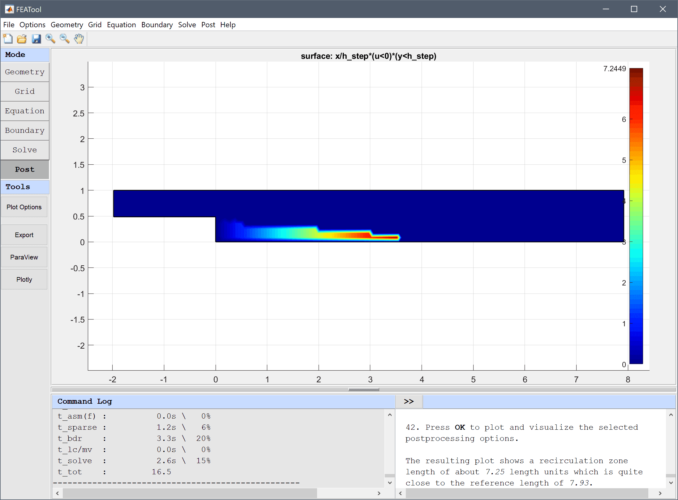
These types of switch expressions can be used to build quite complex expressions and coefficients, for example in the flow over a backwards facing step model the recirculation region is highlighted and visualized with the postprocessing expression x/hstep*(u<0)*(y<0). This expression effectively isolates the region in y < 0 where the x-velocity u is negative, and overlays it with the scaled coordinate x/hstep, resulting in the following plot
Abruptly varying and discontinuous functions like these can sometimes introduce numerical instabilities if used in equation and boundary conditions. From the perspective of the solver it might then be preferable to use a regularized or smoothed Heaviside function, such as
(abs(w)<1)*(1-(0.5*(1+w+1/pi*sin(pi*w)))) + (w<-1)
or a smoothed Dirac delta function
(w>-1 & w<1)*15/16*(1-2*w^2+w^4)/h_grid
where w is a weighting function defining the transition and width of the smoothed region. For example, with w = (sqrt(x^2+y^2)-0.5)/(2*h_grid) a circle with radius 0.5 and transition region width 2*h_grid is defined as shown below.
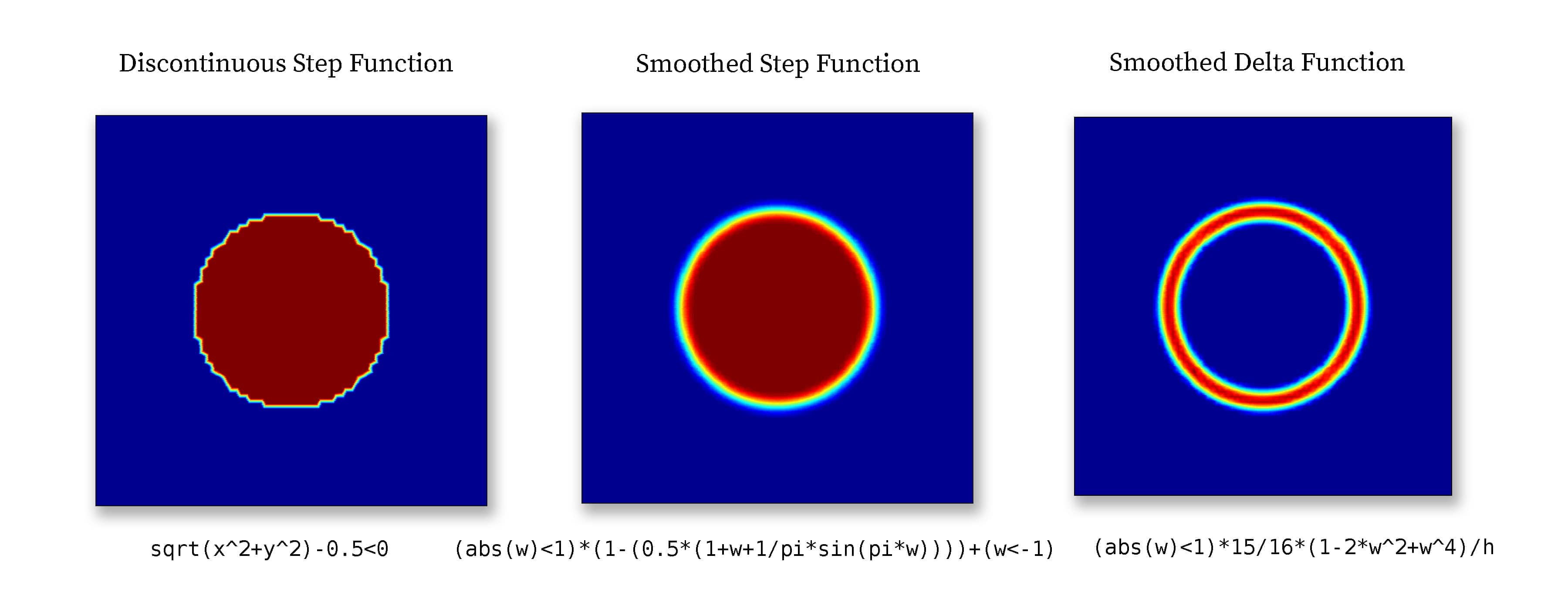
Smoothed step and delta functions are commonly used in models with moving and immersed boundaries which cannot be resolved by the mesh. Step functions are used to define the discontinuous materials, and delta functions to define surface tension forces and reactions. For example see the multiphase flow models ex_multiphase1.
All of the common built-in [mathematical functions and constants in MATLAB](https://www.mathworks.com/help/matlab/elementary-math.html**, such as pi, eps, sqrt, sin, cos, log, exp, abs etc., may also be used to compose expressions.
In cases where coefficients are to be interpolated from tabulated data, it is possible to use the finterpn function. In this case the data must be available as space (txt), comma separated (CSV) ASCII text files, or Mircrosoft Excel format (xls, xlsx) where each column represents data points or values (last column), for example a 3-dimensional interpolation table could look like the following (with 2x3xN interpolation points in the x, y, and z-directions ordered according to ndgrid, respectively)
  x1, y1, z1, v1
  x2, y1, z1, v2
  x1, y2, z1, v3
  x2, y2, z1, v4
  x1, y3, z1, v5
  x2, y3, z1, v6
        ...
  x1, y1, zN, vM-5
        ...
  x2, y3, zN, vM
or alternatively a binary MATLAB .mat file with corresponding data. Tabulated equation and boundary coefficients can for example then be specified as
finterpn('C:\\path_to\\my_tabulated_data.csv',x,T)
where here the full path of the data file is here given as 'C:\path_to\my_tabulated_data.csv' (note the single quotes to specify a string), and interpolation is performed for both x coordinates and the dependent variable T.
A simple heat transfer tutorial example, featuring tabulated the coefficient of heat conductivity (as a function of Temperature) is available in the tutorials section (Heat Conduction with Tabulated Thermal Conductivity).
For more complex coefficients a custom user-defined function can be used as described below.
If a combination of the above methods is insufficient to implement an equation, boundary, or postprocessing expression, or the expression can not be described analytically one can then resort to using a custom MATLAB m-file function.
This could be the case if one wants to use tabulated or experimental data as input which must be interpolated, or complex coefficients with memory effects such as hysteresis. For example, if a equation, boundary, or postprocessing coefficient is entered as myfun(x)
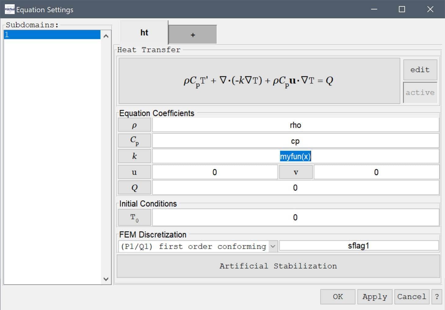
the toolbox parser will first evaluate the inner function arguments (in this case the spatial coordinate x) and then try to find and call the function myfun with these arguments. The function input arguments can be any combination of the valid coefficients described above.
This assumes a function file named myfun.m exists and can be found on any of the MATLAB search paths and directories. By executing the command path on the MATLAB command line will show available directories to save the function in, alternatively a new directory can be added to the search paths with the addpath('path_to_new_folder') command.
The user-defined function must return a numeric array with the same size and dimensions as the input arguments (the function will be called vectorized for performance reasons). A simplified and minimal custom function m-file just returning a constant, could for example look like the following
function [ result ] = myfun( x )
result = 3.14 * ones(size(x));
which would be equivalent to just using the coefficient 3.14 directly.
A more complex example myfun(x,y,t,T) involving the coordinates x, y, time t, and the dependent variable T and interpolation could look something like
function [ result ] = myfun( x, y, t, T )

persistent data_x data_y data_values T0   % Persistent data (assuming they don't change with time).
if( isempty(data_x) )   % Load and define on first run.
   load( 'path_to_mydata_file.mat', 'data_x', 'data_y', 'data_values' );
   T0 = 300;
end

interpolated_data = interp2( data_x, data_y, data_values, x, y );

result = T0 + (1 - cos(2*pi*t)) .* T.^2 .* interpolated_data;

index_limit = find( result < 0 );
result(index_limit) = 0;
In a custom function one can then use the usual MATLAB script functions and techniques such as load (to load external data), save, interp1, interp2, persistent etc. (To see information and syntax about a MATLAB command one can enter help command in the command line interface or see the corresponding MATLAB documentation)
A very advanced example of a custom function evaluating a source term utilizing the evalexpr0 caller arguments is available in the ex_resistive_heating1.m script example.
.* ./ .^ (indicated by the period preceding the operator).The coefficient name h_grid is reserved for the mean grid cell size or diameter, and is defined as the cell_volume^(1/n_sdim), and is primarily used in the artificial and convective stabilization techniques.
Internal and local variables may be prefixed with double underscores __varname, and it is therefore not recommended to name variables with underscores to prevent potential name collisions.
By using the predefined FEATool physics modes it is possible to easily and quickly implement models which simulate different physical effects such as fluid flow, structural stresses, chemical reactions, and heat transfer. This section describes how the various physics modes are defined, set up and used. The available physics modes are listed in the following table
| Physics Mode | Description | Dimensions | Function Definition |
|---|---|---|---|
| Heat Transfer | |||
| Heat Transfer | Conjugate and convective heat transfer | 1D, 2D, 3D | heattransfer |
| Mass Transport | |||
| Convection and Diffusion | Convection, diffusion, and reaction | 1D, 2D, 3D | convectiondiffusion |
| Fluid Dynamics | |||
| Incompressible Flows | |||
| Navier-Stokes Equations | Incompressible fluid flows | 2D, 3D | navierstokes |
| Non-Newtonian Flow | Non-Newtonian and nonlinear fluids | 2D, 3D | nonnewtonian |
| Swirl Flow | Axisymmetric swirling flows | 2D | swirlflow |
| Compressible Flows | |||
| Compressible Flow | Compressible supersonic flows | 2D, 3D | compressibleflow |
| Euler Equations | Inviscid compressible high Ma flows | 1D, 2D, 3D | compressibleeuler |
| Flow in Porous Media | |||
| Darcy's Law | Darcy's law | 2D, 3D | darcyslaw |
| Brinkman Equations | Brinkman equations | 2D, 3D | brinkmaneqns |
| Structural Mechanics | |||
| Euler-Bernoulli Beam | Euler-Bernoulli beam theory | 1D | eulerbeam |
| Plane Stress | Plane stress approximation | 2D | planestress |
| Plane Strain | Plane strain approximation | 2D | planestrain |
| Axisymmetric Stress-Strain | Stress-strain in cylindrical coordinates | 2D | axistressstrain |
| Solid Stress-Strain | Solid stress-strain | 3D | linearelasticity |
| Electromagnetics | |||
| Conductive Media DC | Electric potential | 2D, 3D | conductivemediadc |
| Electrostatics | Electrostatics | 2D, 3D | electrostatics |
| Magnetostatics | Magnetostatics | 2D, 3D | magnetostatics |
| Multiphysics | |||
| Fluid-Structure Interaction | Fluid-structure interaction | 2D, 3D | fluidstructure |
| Classic PDE | |||
| Poisson Equation | Poisson equation | 1D, 2D, 3D | poisson |
| Custom Equation | User defined PDE equations | 1D, 2D, 3D | customeqn |
The equation parameters and coefficients for each selected physics mode are defined in the corresponding Equation Settings dialog boxes described below. In addition to also displaying the PDE equation, it is possible to change or edit the equation definitions with the edit equation button, and activate/deactivate physics modes in specific subdomains with the active button. Furthermore, the used finite element shape functions can also be selected either from the drop down box or directly entering a space separated list of shape functions for each dependent variable. Physics modes with convective effects allowing for numerical artificial stabilization also feature a button opening the stabilization settings.
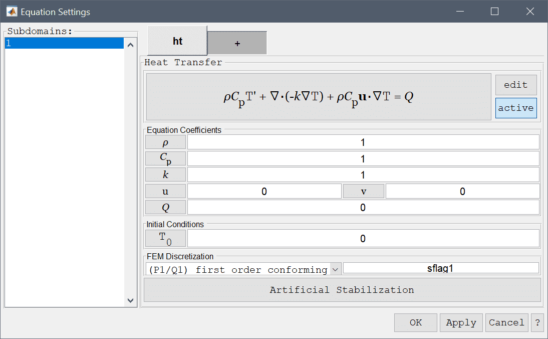
The heat transfer physics mode models heat transport through convection and conduction and heat generation through the following governing equation
\[ \rho C_p\frac{\partial T}{\partial t} + \nabla\cdot(-k\nabla T) + \rho C_p\mathbf{u}\cdot\nabla T = Q \]
where \(\rho\) is the density, \(C_p\) the heat capacity, \(k\) is the thermal conductivity, \(Q\) is the heat source term, and \(\mathbf{u}\) a vector valued convective velocity field. In the Equation Settings dialog box show below the equation coefficients, initial value for the temperature \(T_0 = T(t=0)\) can be specified. The FEM shape function space can also be selected from the drop-down combobox (1st through 5th order conforming P1/Q1 shape functions), or further specified in the corresponding edit field.
For heat transfer problems with dominating convective effects it is advisable to use artificial stabilization. Pressing the lower Artificial Stabilization button opens the corresponding dialog box which allows adding isotropic artificial diffusion, anisotropic streamline diffusion, and shock capturing stabilization. Turning coefficients are also provided to control the strength of the introduced artificial diffusion.
The heat transfer physics mode allows for four different boundary conditions; prescribed temperature, convective flow (outflow condition), an insulation/symmetry condition which prescribes zero flux (or flow), and a prescribed flux boundary condition.
The heat flux boundary condition involves several parameters. Firstly, an arbitrary expression for the heat flux may be prescribed with the coefficient q0. The second term, h*(Tinf-T), represents natural convection between the boundary and the surroundings. Here h is the convective heat transfer coefficient and Tinf a reference bulk temperature. The final term, Const*(Tamb^4-T^4), represents a radiation flux boundary condition where Const is the product between the emissivity of the boundary \(\epsilon\) and the Stefan-Bolzmann constant \(\sigma\), and Tamb is the surrounding ambient temperature.
The boundary conditions are summarized in the table below
| Boundary Condition | Definition | Boundary Coefficient |
|---|---|---|
| Temperature | Prescribed temperature, \(T = T_0\) | T0 |
| Convective flux | Outflow, \(-\mathbf{n}\cdot k\nabla T = 0\) | |
| Thermal insulation/symmetry | Zero heat flux, \(-\mathbf{n}\cdot (k\nabla T + \rho C_p\mathbf{u}c) = 0\) | |
| Heat flux | Prescribed heat flux, \(-\mathbf{n}\cdot (k\nabla T + \rho C_p\mathbf{u}T) = q_0 + h\cdot(T_{inf}-T) + Const\cdot(T_{amb}^4-T^4)\) | q0, h, Tinf, Const, Tamb |
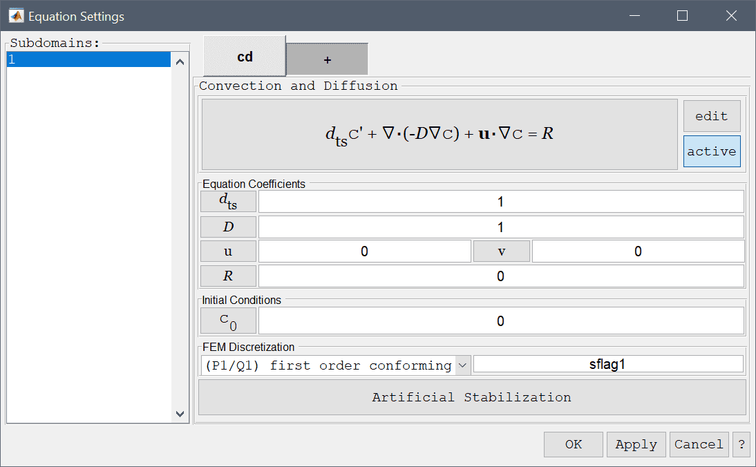
The convection and diffusion physics mode models mass transport and reaction of a chemical species \(c\). The governing equation for convection and diffusion reads
\[ d_{ts}\frac{\partial c}{\partial t} + \nabla\cdot(-D\nabla c) + \mathbf{u}\cdot\nabla c = R \]
where \(d_{ts}\) is a time scaling coefficient, \(D\) is a diffusion coefficient, \(R\) is the reaction rate source term, and \(\mathbf{u}\) a vector valued convective velocity field. In the Equation Settings dialog box shown below these equation coefficients, initial value \(c_0 = c(t=0)\) can be specified. The FEM shape function space can also be selected from the drop-down combobox (1st through 5th order conforming P1/Q1 shape functions), or further specified in the corresponding edit field.
For convection and diffusion problems with dominating convective effects it is advisable to use artificial stabilization. Pressing the lower Artificial Stabilization button opens the corresponding dialog box which allows adding isotropic artificial diffusion, anisotropic streamline diffusion, and shock capturing stabilization. Turning coefficients are also provided to control the strength of the introduced artificial diffusion.
The convection and diffusion physics mode allows for four different boundary conditions; a prescribed concentration boundary condition, a convective flow (outflow condition), an insulation/symmetry condition which prescribes zero flux (or flow), and a prescribed flux condition. These boundary conditions are summarized in the table below
| Boundary Condition | Definition | Boundary Coefficient |
|---|---|---|
| Concentration | Prescribed concentration, \(c = c_0\) | c0 |
| Convective flux | Outflow, \(-\mathbf{n}\cdot D\nabla c = 0\) | |
| Insulation/symmetry | Zero flux/flow, \(-\mathbf{n}\cdot (D\nabla c + \mathbf{u}c) = 0\) | |
| Flux condition | Prescribed flux, \(-\mathbf{n}\cdot (D\nabla c + \mathbf{u}c) = N_0\) | N0 |
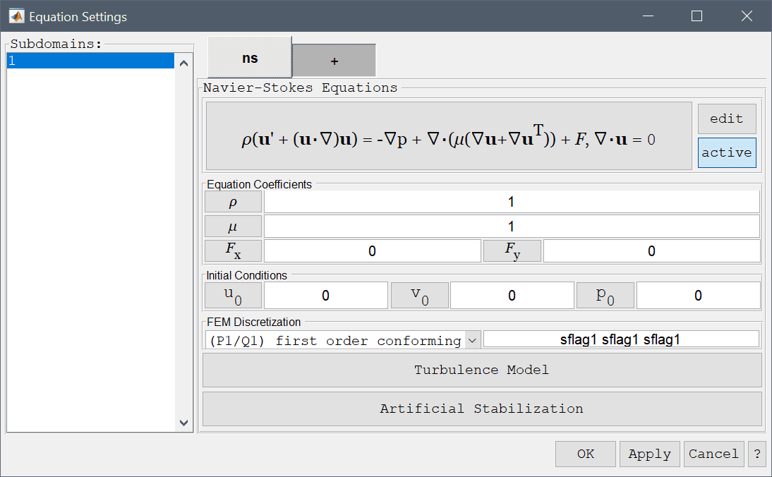
The Navier-Stokes equations physics mode models flows of incompressible fluid flows and which is described by
\[ \left\{\begin{aligned} \rho\left( \frac{\partial\mathbf{u}}{\partial t} + (\mathbf{u}\cdot\nabla)\mathbf{u}\right) - \nabla\cdot(\mu(\nabla\mathbf{u}+\nabla\mathbf{u}^T)) + \nabla p &= \mathbf{F} \\ \nabla\cdot\mathbf{u} &= 0 \end{aligned}\right. \]
which is to be solved for the unknown velocity field \(\mathbf{u}\) and pressure \(p\). In these equations \(\rho\) represents the density of the fluid and \(\mu\) the dynamic viscosity, moreover \(\mathbf{F}\) represents body forces acting on the fluid. In the Equation Settings dialog box shown below the equation coefficients, initial values for the velocities and pressures can be specified. The FEM shape function spaces can also be selected from the drop-down combobox (P2P1/Q2Q1 and P1P-1/Q2P1 shape functions), or further specified in the corresponding edit field.
Turbulent effects must often be approximated due to limited mesh resolution. This can be achieved by using a Turbulence Model, pressing the corresponding button button opens a dialog box where the allows a turbulence model to be selected. See the Turbulence Modeling Section "turbulence" on more information about turbulence models.
For flow problems with dominating convective effects it is advisable to use artificial stabilization. Pressing the lower Artificial Stabilization button opens the corresponding dialog box which allows adding isotropic artificial diffusion, anisotropic streamline diffusion, shock capturing, and pressure stabilization (for first order discretizations). Turning coefficients are also provided to control the strength of the introduced artificial diffusion.
The Navier-Stokes equations physics mode allows prescription of several different boundary conditions. Firstly, the no-slip (zero velocity) boundary condition which is appropriate for stationary walls. Moreover, a prescribed velocity condition can be prescribed to both in and outflows as well as moving walls. Prescribed pressure and neutral (zero viscous stress) conditions are both appropriate for outflows. Lastly, symmetry or slip conditions sets the flow to zero in the normal direction so as to prevent flow normal to the boundary. These boundary conditions are summarized in the table below
| Boundary Condition | Definition | Boundary Coefficient |
|---|---|---|
| Wall/no-slip | Zero velocity, \(\mathbf{u} = 0\) | |
| Inlet/velocity | Prescribed velocity, \(\mathbf{u} = (u_0, v_0, w_0)\) | u0, v0, w0 |
| Neutral outflow/stress boundary | Zero stress, \(-\mathbf{n}\cdot (-p\mathbf{I} + \mu(\nabla\mathbf{u}+\nabla\mathbf{u}^T)) = 0\) | |
| Outflow/pressure | Prescribed pressure, \(p = p_0\) | p0 |
| Symmetry/slip | Zero normal velocity, \(\mathbf{n}\cdot\mathbf{u} = 0\) |
The non-Newtonian flow physics mode is an extension of Navier-Stokes equations which allows for several predefined non-Newtonian viscosity formulations.
In the Equation Settings dialog box shown below the viscosity model can be selected between power law, Bird-Carreau, Cross power law, and custom models. Selecting a model in the drop down menu will update the corresponding viscosity expression, \(\mu\).
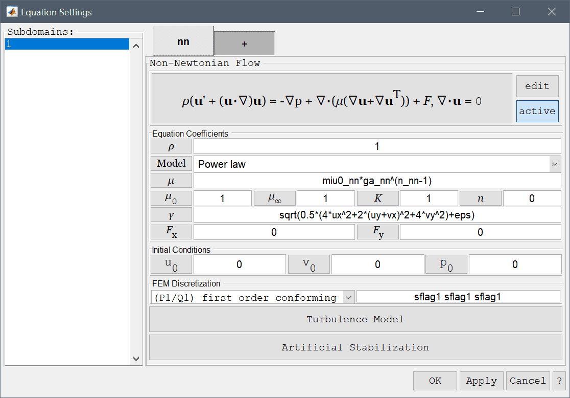
The power law or Oswald model represents the viscosity as an exponential function of the shear rate \(\dot{\gamma}\)
\[ \mu = \mu_0\dot{\gamma}^{n-1} \]
where \(\mu_0\) is the flow consistency index, and \(n\) the flow behavior index. For 0 < n < 1 the fluid shows shear thinning or pseudo-plastic behavior, n = 1 is Newtonian flow, and for n > 1 the fluid shows shear thickening (dilatant) behavior. This model is suitable for for shear-thinning flows, such as in relatively mobile fluids, for example in low-viscosity dispersions and weak gels.
The Bird-Carreau model is a model bounded by the viscosities at zero \(\mu_0\) (Newtonian) and infinity \(\mu_\infty\) shear rates (such as in blade, knife and roller coating processes).
\[ \mu = \mu_\infty + (\mu_0 - \mu_\infty)(1 + (K\dot{\gamma})^2)^{(n-1)/2} \]
Here \(K\) is the relaxation time, and n the power index.
The Cross power law model covers the full shear thinning region through the formula
\[ \mu = \mu_\infty + \frac{\mu_0 - \mu_\infty}{1 + (K\dot{\gamma})^n} \]
here \(\mu_0\) and \(\mu_\infty\) are the viscosity at zero infinity shear rates. The parameter \(K\) is the cross time constant, where the reciprocal, \(1/K\), gives the critical shear rate at which the onset of shear thinning can occur. Finally, \(n\) the dimensionless cross rate index or constant, which prescribes how the viscosity depends on the shear rate (going from zero Newtonian, to unity for increasing shear thinning behavior).
The custom model allows the user to enter any user defined expression, and can use the expression for the shear or strain rate \(\dot{\gamma}\).
The model and equation coefficients, and initial values for the velocities and pressures can also be specified. The FEM shape function spaces can also be selected from the drop-down combobox (P2P1/Q2Q1 and P1P-1/Q2P1 shape functions), or further specified in the corresponding edit field.
Boundary conditions, turbulence, artificial stabilization settings are identical to those of the Navier-Stokes equations.
The swirl flow physics mode is an extension of Axisymmetric Navier-Stokes equations which allows for non-zero azimuthal velocity (swirl effects). The 2D physics mode allows for a three dimensional velocity field with corresponding momentum equations.
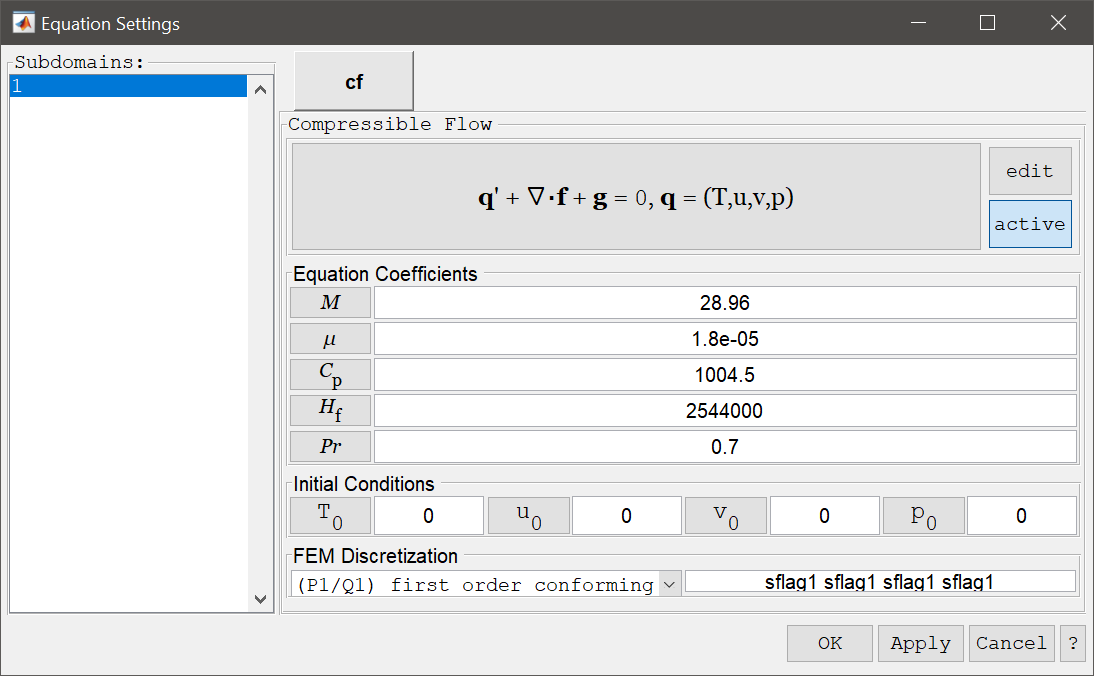
The compressible flow physics mode is used to model and simulate supersonic high Mach (Ma) numer and transsonic viscous flows of compressible ideal gases, including turbulent effects.
The compressible flow equations for viscous compressible gases is described by
\[ \left\{\begin{aligned} & \frac{\partial\rho}{\partial t} + \nabla\cdot(\rho\mathbf{u}) = 0 \\ & \rho\frac{\partial\mathbf{u}}{\partial t} + \rho(\mathbf{u}\cdot\nabla)\mathbf{u} + \nabla\cdot(p\mathbf{I} - \tau) = \mathbf{0} \\ & \rho C_p(\frac{\partial T}{\partial t} + (\mathbf{u}\cdot\nabla)T) - \tau:\frac{1}{2}(\nabla\mathbf{u}+\nabla\mathbf{u}^T) + \frac{T}{\rho}\frac{\partial \rho}{\partial T}|_p(\frac{\partial p}{\partial t} + (\mathbf{u}\cdot\nabla)p) = 0 \end{aligned}\right. \]
which is to be solved for the dependent variables density \(\rho\), temperature \(T\), velocity field \(\mathbf{u}\) and pressure \(p\), and where \(\tau\) is the viscous stress tensor.
The fluid parameters are specified in the Equation Settings dialog box, specifically the Molecular weight M, dynamic viscosity \(\mu\), Heat capacity at constant pressure \(C_p\), Heat of fusion \(H_f\), and the Prandtl number Pr, and initial conditions of the temperature, velocity, and pressure fields.
Compressible viscous flow problems can currently only be solved with the external OpenFOAM CFD solver using either the rhoCentralFoam or sonicFoam solvers (and therefor is not possible to use as a coupled multi-physics model). In addition turbulence effects using Reynolds Average Navier-Stokes (RAS) models such as the k-Epsilon can also be used with the OpenFOAM solver.
The compressible flow physics mode supports the boundary conditions listed in the table below.
| Boundary Condition | Definition | Boundary Coefficient |
|---|---|---|
| Wall/no-slip | Zero velocity, \(\mathbf{u} = 0\) | |
| Free stream/slip | Free stream values, \(T,\mathbf{u},p = T_0,\mathbf{u}_0,p_0\) | T0, u0, v0, w0, p0 |
| Fixed values/inlet | Prescribed values, \(T,\mathbf{u},p = T_0,\mathbf{u}_0,p_0\) | T0, u0, v0, w0, p0 |
| Neutral/no stress boundary/outlet | Zero stress boundary, \(\partial\phi\partial n = 0\) | |
| Outlet/inlet boundary | Neutral outflow, \(\partial\phi\partial n = 0\) or prescribed inflow, \(T,\mathbf{u},p = T_0,\mathbf{u}_0,p_0\) | T0, u0, v0, w0, p0 |
| Symmetry | Zero normal velocity, \(\mathbf{n}\cdot\mathbf{u} = 0\) |
The Wall/no-slip condition prescribe zero-velocity on walls, while the Fixed values/inlet boundary conditions is used to exactly prescribe flow variables on inlets and outlets. Free stream/slip is used on to prescribe a supersonic free-stream condition where the Prandtl-Meyer expansion is used in case of inflow with the specified far away flow variables, or in case of outflow a zero-gradient condition is applied. The Neutral/no stress boundary/outlet condition prescribes a zero gradient for all variables suitable for some outlet boundaries, where in contrast the Outlet/inlet boundary condition prescribes zero gradient in case of flow outwards from the boundary, and the prescribed coefficients in case of inflow. Lastly the Symmetry boundary condition can be applied to boundaries which should be mirror symmetric.
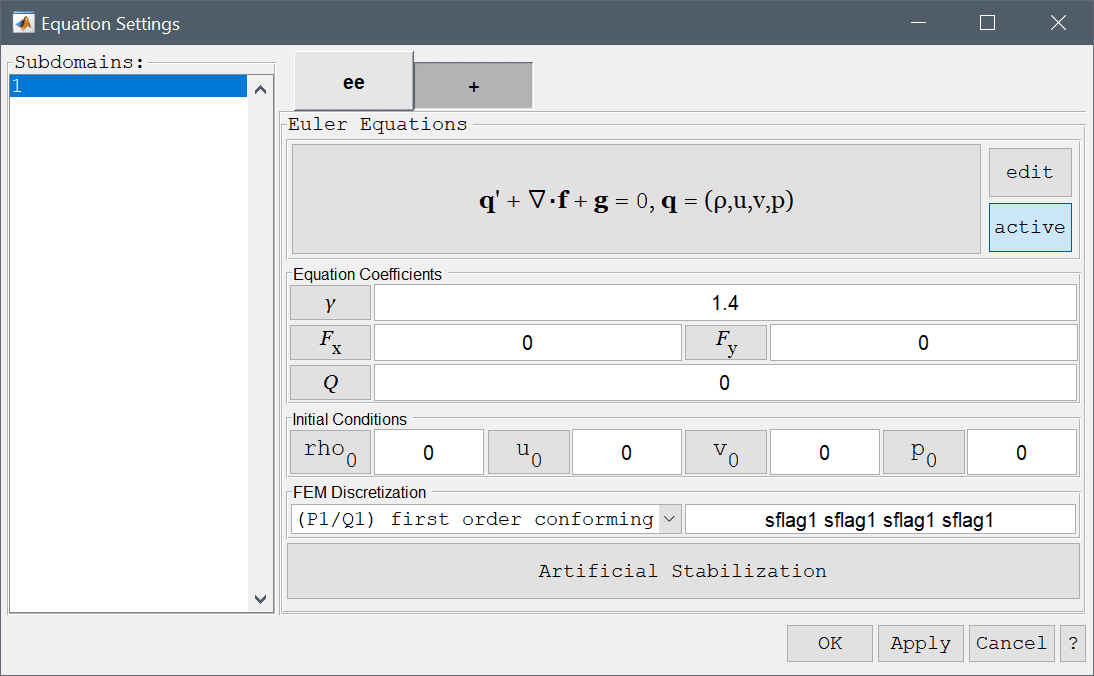
The Euler equations for inviscid compressible flows is described by
\[ \left\{\begin{aligned} & \frac{\partial\rho}{\partial t} + (\mathbf{u}\cdot\nabla)\rho + \rho(\nabla\cdot\mathbf{u}) = 0 \\ & \frac{\partial\mathbf{u}}{\partial t} + (\mathbf{u}\cdot\nabla)\mathbf{u} + \frac{1}{\rho}\nabla p = \frac{1}{\rho}\mathbf{F} \\ & \frac{\partial p}{\partial t} + (\mathbf{u}\cdot\nabla)p + \gamma p(\nabla\cdot\mathbf{u}) = (\gamma-1)(Q-(\mathbf{F}\cdot\mathbf{u})) \end{aligned}\right. \]
which is to be solved for the primitive variables density \(\rho\), velocity field \(\mathbf{u}\) and pressure \(p\). In the Equation Settings dialog box shown below the ratio of specific heats \(\gamma\), source terms F and Q, and initial values for the density, velocities, and pressures can be specified. The FEM shape function spaces can also be selected from the drop-down combobox, or further specified in the corresponding edit field.
As inviscid flow problems to not feature stabilizing viscosity and also may feature discontinous shocks it is neccessary to add artificial stabilization. Pressing the lower Artificial Stabilization button opens the corresponding dialog box which allows adding isotropic artificial diffusion, anisotropic streamline diffusion, and shock capturing. Turning coefficients are also provided to control the strength of the introduced artificial diffusion.
The compressible Euler equations physics mode allows prescription of either all the dependent variables for inlets and outlets, symmetry/slip conditions with zero normal velocity, and a neutral/no stress condition appropriate for outlets. These boundary conditions are summarized in the table below
| Boundary Condition | Definition | Boundary Coefficient |
|---|---|---|
| Inlet/outlet | Prescribed variables, \(\rho = \rho_0,\ \mathbf{u} = (u_0, v_0, w_0),\ p = p_0\) | rho0, u0, v0, w0, p0 |
| Symmetry/slip | Zero normal velocity, \(\mathbf{n}\cdot\mathbf{u} = 0\) | |
| Neutral/no stress boundary/outlet | Zero stress boundary |
Darcy's law models the pressure p in porous media flow through the relation
\[ d_{ts}\frac{\partial p}{\partial t} + \nabla\cdot(-\frac{\kappa}{\eta}\nabla p) = F \]
where \(\kappa\) represents permeability, \(\eta\) viscosity, F sources and sinks, and \(d_{ts}\) is a time scaling coefficient. In the Darcy's Law Equation Settings dialog box shown below the equation coefficients, initial values for the pressure can be specified. The FEM shape function spaces can also be selected from the drop-down combobox, or further specified in the corresponding edit field.

The Darcy's law physics mode allows prescription of three different boundary conditions. The prescribed pressure, flux, and insulation boundary conditions are summarized in the table below
| Boundary Condition | Definition | Boundary Coefficient |
|---|---|---|
| Pressure | Prescribed pressure, \(\mathbf{p} = p_0\) | p0 |
| Insulation/symmetry | Zero flux/flow, \(-\mathbf{n}\cdot(-\frac{\kappa}{\eta}\nabla p) = 0\) | |
| Flux | Prescribed flux/flow, \(-\mathbf{n}\cdot(-\frac{\kappa}{\eta}\nabla p) = N_0\) | N0 |
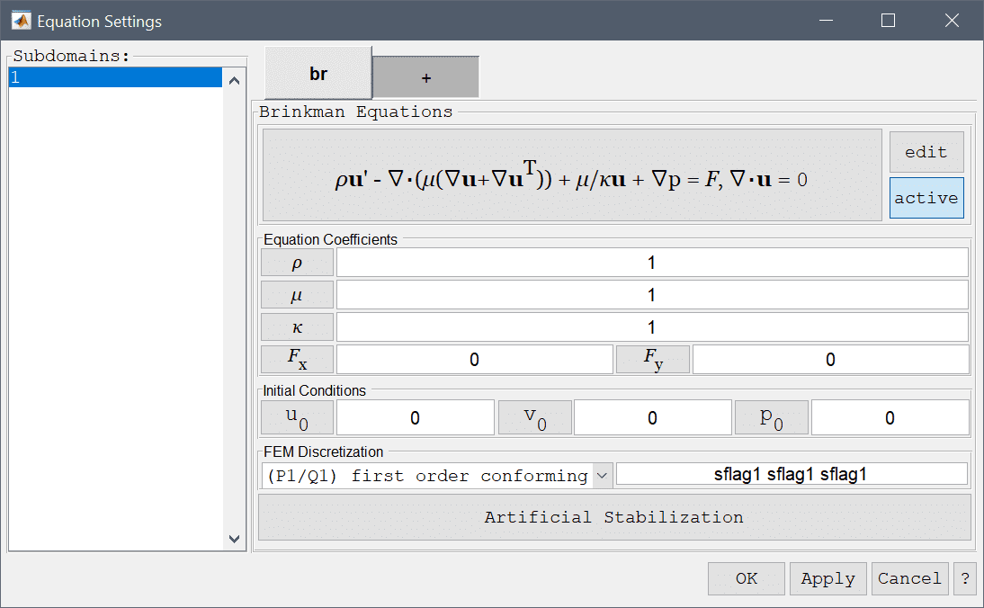
The Brinkman equations physics mode models porous media flows and can be seen as a combination of Darcy's law with the Navier-Stokes equations. The Brinkman equations are defined as follows
\[ \left\{\begin{aligned} \rho\frac{\partial\mathbf{u}}{\partial t} - \nabla\cdot(\mu(\nabla\mathbf{u}+\nabla\mathbf{u}^T)) + \frac{\mu}{\kappa}\mathbf{u} + \nabla p &= \mathbf{F} \\ \nabla\cdot\mathbf{u} &= 0 \end{aligned}\right. \]
which is to be solved for the unknown velocity field \(\mathbf{u}\) and pressure \(p\). In these equations \(\rho\) represents the density of the fluid, \(\mu\) the viscosity, and \(\kappa\) permeability, moreover \(\mathbf{F}\) represents body forces acting on the fluid. In the Equation Settings dialog box shown below the equation coefficients, initial values for the velocities and pressures can be specified. The FEM shape function spaces can also be selected from the drop-down combobox (P2P1/Q2Q1 and P1P-1/Q2P1 shape functions), or further specified in the corresponding edit field.
The Brinkman equations physics mode allows prescription of several different boundary conditions. Firstly, the no-slip (zero velocity) boundary condition which is appropriate for stationary walls. Moreover, a prescribed velocity condition can be prescribed to both in and outflows as well as moving walls. Prescribed pressure and neutral (zero viscous stress) conditions are both appropriate for outflows. Lastly, symmetry or slip conditions sets the flow to zero in normal direction so as to prevent flow normal to the boundary. These boundary conditions are summarized in the table below
| Boundary Condition | Definition | Boundary Coefficient |
|---|---|---|
| Wall/no-slip | Zero velocity, \(\mathbf{u} = 0\) | |
| Inlet/velocity | Prescribed velocity, \(\mathbf{u} = (u_0, v_0, w_0)\) | u0, v0, w0 |
| Neutral outflow/stress boundary | Zero stress, \(-\mathbf{n}\cdot (-p\mathbf{I} + \mu(\nabla\mathbf{u}+\nabla\mathbf{u}^T)) = 0\) | |
| Outflow/pressure | Prescribed pressure, \(p = p_0\) | p0 |
| Symmetry/slip | Zero normal velocity, \(\mathbf{n}\cdot\mathbf{u} = 0\) |
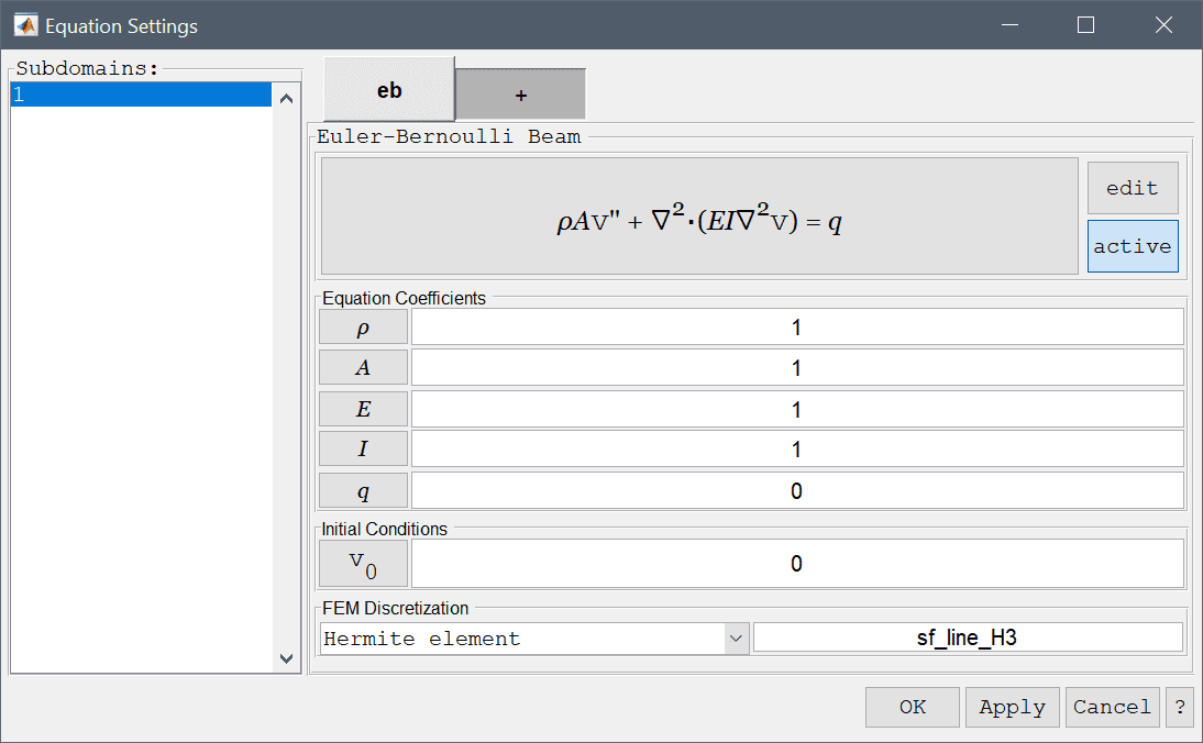
The Euler-Bernoulli beam physics mode models displacements, stresses and strains in a one-dimensional representations of beams and bars. The Euler-Bernoulli equations for the displacement \(v\) reads
\[ \rho A \frac{\partial^2 v}{\partial t^2} + \frac{\partial^2}{\partial x^2}(EI\frac{\partial^2 v}{\partial x^2}) = q \]
where \(\rho\) is the beam material density, A the cross-sectional area, E modulus of elasticity, I cross section moment of inertia, and q any distributed loads. In the Euler beam Equation Settings dialog box shown below these equation coefficients, initial value \(v_0 = v(t=0)\) can be specified. The FEM shape function space can also be selected from the drop-down combobox (Hermite C1 shape functions by default).
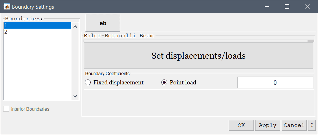
The boundary conditions for the Euler beam physics mode allows for any combination of prescribing displacements and edge loads. These boundary conditions are summarized in the table below.
| Boundary Condition | Definition | Boundary Coefficient |
|---|---|---|
| Fixed displacements | Prescribed displacements, \( u = u_0, v = v_0\) | v0 |
| Edge loads | Prescribed edge loads, \( F_x = f_{x,0}, F_y = f_{y,0} \) | fy,0 |
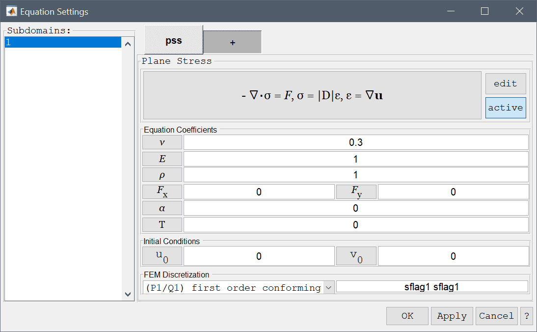
The plane stress physics mode models how structural stresses form in thin structures where the planar component of the stress can be neglected or considered zero. In this case the stress-strain relations can be written as
\[ \left( \begin{array}{c} \sigma_x \\ \sigma_y \\ \tau_{xy} \end{array} \right) = \frac{E}{1-\nu^2} \left(\begin{array}{ccc} 1 & \nu & 0 \\ \nu & 1 & 0 \\ 0 & 0 & \frac{1-\nu}{2} \end{array} \right) \left( \begin{array}{c} \epsilon_x \\ \epsilon_y \\ \gamma_{xy} \end{array} \right) \]
where \(E\) is the elastic or Young's modulus, and \(\nu\) is the Poisson's ratio of the material. The strains are related to the material displacements ( \(u\), \(v\)) as
\[ \epsilon_x = \frac{\partial u}{\partial x}, \qquad \epsilon_y = \frac{\partial v}{\partial y}, \qquad \gamma_{xy} = \frac{\partial u}{\partial y} + \frac{\partial v}{\partial x} \]
Balance equations for the stresses finally give the resulting governing equation system as
\[ \left\{\begin{aligned} - \frac{\partial\sigma_x}{\partial x} - \frac{\partial\tau_{xy}}{\partial y} = F_x \\ - \frac{\partial\tau_{xy}}{\partial x} - \frac{\partial\sigma_y}{\partial y} = F_y \end{aligned}\right. \]
where \(F_x\) and \(F_y\) are volume (body) forces in the x and y-directions, respectively. In the Equation Settings dialog box shown below the equation coefficients, initial value for the displacements can be specified. The FEM shape function space can also be selected from the drop-down combobox (1st through 5th order conforming P1/Q1 shape functions), or further specified in the corresponding edit field.
Optional stress-strain temperature dependence can also be added, which takes the form
\[ \mathbf{\sigma} = \mathbf{D\epsilon} - \frac{E\alpha T}{1-\nu}[1\ \ 1\ \ 0]^T \]
where \(\alpha\) is the coefficient of thermal expansion and \(T\) either a prescribed temperature field, a dependent variable name from another physics mode that represents the temperature, or a combination such as \(T-T_{ref}\).
The boundary conditions for the plane stress physics mode allows for any combination of prescribing displacements and edge loads. These boundary conditions are summarized in the table below.
| Boundary Condition | Definition | Boundary Coefficient |
|---|---|---|
| Fixed displacements | Prescribed displacements, \( u = u_0, v = v_0\) | u0, v0 |
| Edge loads | Prescribed edge loads, \( F_x = f_{x,0}, F_y = f_{y,0} \) | fx,0, fy,0 |
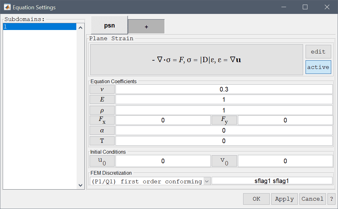
Like the plane stress physics mode, the plane strain mode models how structural stresses form in structures but where the z-component of the displacements can be neglected or considered zero. In this case the stress-strain relations can be written as
\[ \left( \begin{array}{c} \sigma_x \\ \sigma_y \\ \tau_{xy} \end{array} \right) = \frac{E}{(1+\nu)(1-2\nu)} \left(\begin{array}{ccc} {1-\nu} & \nu & 0 \\ \nu & {1-\nu} & 0 \\ 0 & 0 & \frac{1-2\nu}{2} \end{array}\right) \left( \begin{array}{c} \epsilon_x \\ \epsilon_y \\ \gamma_{xy} \end{array} \right) \]
where \(E\) is the elastic or Young's modulus, and \(\nu\) is the Poisson's ration of the material. The strains are related to the material displacements ( \(u\), \(v\)) as
\[ \epsilon_x = \frac{\partial u}{\partial x}, \qquad \epsilon_y = \frac{\partial v}{\partial y}, \qquad \gamma_{xy} = \frac{\partial u}{\partial y} + \frac{\partial v}{\partial x} \]
Balance equations for the stresses finally give the resulting governing equation system as
\[ \left\{\begin{aligned} - \frac{\partial\sigma_x}{\partial x} - \frac{\partial\tau_{xy}}{\partial y} = F_x \\ - \frac{\partial\tau_{xy}}{\partial x} - \frac{\partial\sigma_y}{\partial y} = F_y \end{aligned}\right. \]
where \(F_x\) and \(F_y\) are volume (body) forces in the x and y-directions, respectively. In the Equation Settings dialog box shown below the equation coefficients, initial value for the displacements can be specified. The FEM shape function space can also be selected from the drop-down combobox (1st through 5th order conforming P1/Q1 shape functions), or further specified in the corresponding edit field.
Optional stress-strain temperature dependence can also be added, which takes the form
\[ \mathbf{\sigma} = \mathbf{D\epsilon} - \frac{E\alpha T}{(1+\nu)(1-2\nu)}[1\ \ 1\ \ 0]^T \]
where \(\alpha\) is the coefficient of thermal expansion and \(T\) either a prescribed temperature field, a dependent variable name from another physics mode that represents the temperature, or a combination such as \(T-T_{ref}\).
The boundary conditions for the plane strain physics mode allows for any combination of prescribing displacements and edge loads. These boundary conditions are summarized in the table below.
| Boundary Condition | Definition | Boundary Coefficient |
|---|---|---|
| Fixed displacements | Prescribed displacements, \( u = u_0, v = v_0\) | u0, v0 |
| Edge loads | Prescribed edge loads, \( F_x = f_{x,0}, F_y = f_{y,0} \) | fx,0, fy,0 |
The axisymmetric stress-strain physics mode models how stresses and strains in cylindrical and rotationally symmetric geometries behave. The model equations are reduced from full 3D to a two-dimensional slice. In this case the balance equations for stress-strain (valid for the half plane r>0, with r=0 being the symmetry axis) can be written as
\[ \left\{\begin{aligned} - \frac{\partial\sigma_r}{\partial r} - \frac{\partial\tau_{rz}}{\partial z} - \frac{\sigma_r - \sigma_\theta}{r} = F_r \\ - \frac{\partial\tau_{rz}}{\partial r} - \frac{\partial\sigma_z}{\partial z} - \frac{\tau_{rz}}{r} = F_z \end{aligned}\right. \]
where \(F_r\) and \(F_z\) are volume (body) forces in the r and z-directions, respectively. The balance equations together with the constitutive relations
\[ \left( \begin{array}{c} \sigma_r \\ \sigma_\theta \\ \sigma_z \\ \tau_{rz} \end{array} \right) = \frac{E\nu}{(1+\nu)(1-2\nu)} \left(\begin{array}{cccc} \frac{1-\nu}{\nu} & 1 & 1 & 0 \\ 1 & \frac{1-\nu}{\nu} & 1 & 0 \\ 1 & 1 & \frac{1-\nu}{\nu} & 0 \\ 0 & 0 & 0 & \frac{1-2\nu}{2\nu} \end{array} \right) \left( \begin{array}{c} \epsilon_r \\ \epsilon_\theta \\ \epsilon_z \\ \gamma_{rz} \end{array} \right) \]
uniquely define the equations to solve. Here \(E\) is the elastic or Young's modulus, and \(\nu\) is the Poisson's ratio of the material. The strains are related to the material displacements ( \(u\), \(w\)) as
\[ \epsilon_r = \frac{\partial u}{\partial r}, \qquad \epsilon_\theta = \frac{u}{r}, \qquad \epsilon_z = \frac{\partial w}{\partial z}, \qquad \gamma_{rz} = \frac{\partial u}{\partial z} + \frac{\partial w}{\partial r} \]
In the PDE equation formulations the dependent variable u is replaced by u/r in order to avoid divisions by zero on the symmetry line (Thus custom postprocessing expressions including u should instead use r*u).
In the Equation Settings dialog box shown below the equation coefficients, initial value for the displacements can be specified. The FEM shape function space can also be selected from the drop-down combobox (1st through 5th order conforming P1/Q1 shape functions), or further specified in the corresponding edit field.

Optional stress-strain temperature dependence can also be added, which takes the form
\[ \mathbf{\sigma} = \mathbf{D\epsilon} - \frac{E\alpha T}{1-\nu}[1\ \ 1\ 1\ \ 0]^T \]
where \(\alpha\) is the coefficient of thermal expansion and \(T\) either a prescribed temperature field, a dependent variable name from another physics mode that represents the temperature, or a combination such as \(T-T_{ref}\).
The boundary conditions for the plane stress physics mode allows for any combination of prescribing displacements and edge loads. These boundary conditions are summarized in the table below.
| Boundary Condition | Definition | Boundary Coefficient |
|---|---|---|
| Fixed displacements | Prescribed displacements, \( u = u_0, w = w_0\) | u0, w0 |
| Edge loads | Prescribed edge loads, \( F_r = f_{r,0}, F_z = f_{z,0} \) | fr,0, fz,0 |
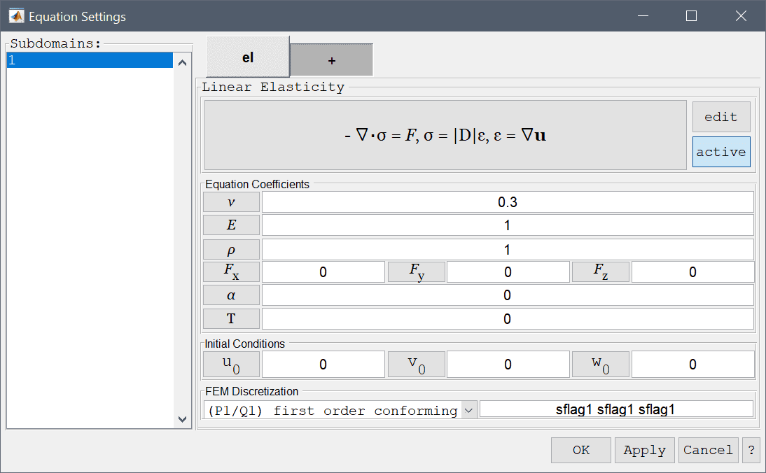
The linear elasticity physics mode models how structural stresses form in solid structures where the stress-strain relations can be written as
\[ \left( \begin{array}{c} \sigma_x \\ \sigma_y \\ \sigma_z \\ \tau_{xy} \\ \tau_{yz} \\ \tau_{xz} \end{array} \right) = \frac{E}{(1+\nu)(1-2\nu)} \left(\begin{array}{cccccc} 1-\nu & \nu & \nu & 0 & 0 & 0 \\ \nu & 1-\nu & \nu & 0 & 0 & 0 \\ \nu & \nu & 1-\nu & 0 & 0 & 0 \\ 0 & 0 & 0 & \frac{1-2\nu}{2} & 0 & 0 \\ 0 & 0 & 0 & 0 & \frac{1-2\nu}{2} & 0 \\ 0 & 0 & 0 & 0 & 0 & \frac{1-2\nu}{2} \end{array} \right) \left( \begin{array}{c} \epsilon_x \\ \epsilon_y \\ \epsilon_z \\ \gamma_{xy} \\ \gamma_{yz} \\ \gamma_{xz} \end{array} \right) \]
where \(E\) is the elastic or Young's modulus, and \(\nu\) is the Poisson's ratio of the material. The strains are related to the material displacements ( \(u\), \(v\), \(w\)) as
\[ \epsilon_x = \frac{\partial u}{\partial x}, \qquad \epsilon_y = \frac{\partial v}{\partial y}, \qquad \epsilon_z = \frac{\partial w}{\partial z}, \qquad \gamma_{xy} = \frac{\partial u}{\partial y} + \frac{\partial v}{\partial x}, \qquad \gamma_{yz} = \frac{\partial v}{\partial z} + \frac{\partial w}{\partial y}, \qquad \gamma_{xz} = \frac{\partial u}{\partial z} + \frac{\partial w}{\partial x} \]
Balance equations for the stresses finally give the resulting governing equation system as
\[ \left\{\begin{aligned} - \frac{\partial\sigma_x}{\partial x} - \frac{\partial\tau_{xy}}{\partial y} - \frac{\partial\tau_{xz}}{\partial z} = F_x \\ - \frac{\partial\tau_{xy}}{\partial x} - \frac{\partial\sigma_y}{\partial y} - \frac{\partial\tau_{yz}}{\partial z} = F_y \\ - \frac{\partial\tau_{xz}}{\partial x} - \frac{\partial\tau_{yz}}{\partial y} - \frac{\partial\sigma_z}{\partial z} = F_z \end{aligned}\right. \]
where \(F_x\), \(F_y\), and \(F_z\) are volume (body) forces in the x, y, and z-directions, respectively. In the Equation Settings dialog box shown below the equation coefficients, initial value for the displacements can be specified. The FEM shape function space can also be selected from the drop-down combobox (1st through 5th order conforming P1/Q1 shape functions), or further specified in the corresponding edit field.
Optional stress-strain temperature dependence can also be added, which takes the form
\[ \mathbf{\sigma} = \mathbf{D\epsilon} - \frac{E\alpha T}{1-2\nu}[1\ \ 1\ \ 1\ \ 0\ \ 0\ \ 0]^T \]
where \(\alpha\) is the coefficient of thermal expansion and \(T\) either a prescribed temperature field, a dependent variable name from another physics mode that represents the temperature, or a combination such as \(T-T_{ref}\).
The boundary conditions for the linear elasticity physics mode allows for any combination of prescribing displacements and edge loads. These boundary conditions are summarized in the table below
| Boundary Condition | Definition | Boundary Coefficient |
|---|---|---|
| Fixed displacements | Prescribed displacements, \( u = u_0, v = v_0, w = w_0\) | u0, v0 , w0 |
| Edge loads | Prescribed edge loads, \( F_x = f_{x,0}, F_y = f_{y,0}, F_z = f_{z,0} \) | fx,0, fy,0, fz,0 |
Electric potential and current can be modeled through the conductive media DC physics mode. To describe the flow of current and electric potential \(V\) an electric field is firstly defined as \(\mathbf{E} = \nabla V\). Furthermore, the current density \(\mathbf{J}\) is related to the electric field by \(\mathbf{J} = \sigma\mathbf{E}\) where \(\sigma\) is the conductivity. By assuming conservation of the current one can pose a continuity equation for the current density, that is \(\nabla\cdot\mathbf{J} = Q\) where \(Q\) is a current source, which after expansion results in the following equation
\[ d_{ts}\frac{\partial V}{\partial t} + \nabla\cdot(-\sigma\nabla V) = Q \]
In the Equation Settings dialog box shown below the equation coefficients, initial value for the electric potential \(V_0 = V(t=0)\) can be specified. The FEM shape function space can also be selected from the drop-down combobox (1st through 5th order conforming P1/Q1 shape functions), or further specified in the corresponding edit field.

The conductive media DC physics mode features two boundary conditions, one prescribing the electric potential at a boundary \(V = V_0\), and the other prescribing the current flow into the boundary. These boundary conditions are summarized in the table below
| Boundary Condition | Definition | Boundary Coefficient |
|---|---|---|
| Electric potential | Prescribed electric potential, \(V = V_0\) | V0 |
| Current flow | Prescribed current flow (flux), \(-\mathbf{n}\cdot (\sigma\nabla V) = J_0\) | J0 |
The electrostatics physics mode is an extension of the conductive media DC mode allowing for polarization vector, P, to be taken into account. The electrostatics equation for the electric potential V then reads
\[ -\nabla\cdot(\epsilon\nabla V - \mathbf{P}) = \rho \]
where \(\epsilon\) is the permittivity and \(\rho\) the charge density source term.
In the Equation Settings dialog box shown below the equation coefficients, initial value for the electric potential \(V_0 = V(t=0)\) can be specified. The FEM shape function space can also be selected from the drop-down combobox (1st through 5th order conforming P1/Q1 shape functions), or further specified in the corresponding edit field.

The electrostatics physics mode features two boundary conditions, one prescribing the electric potential at a boundary \(V = V_0\), and the other prescribing the current flow into the boundary. These boundary conditions are summarized in the table below
| Boundary Condition | Definition | Boundary Coefficient |
|---|---|---|
| Electric potential | Prescribed electric potential, \(V = V_0\) | V0 |
| Ground/antisymmetry | Zero electric potential, \(V = 0\) | |
| Surface charge | Prescribed current flow (flux), \(-\mathbf{n}\cdot (-\epsilon\nabla V + \mathbf{P}) = \rho_s\) | rhos |
| Insulation/symmetry | Zero current flow (flux), \(-\mathbf{n}\cdot (-\epsilon\nabla V + \mathbf{P}) = 0\) |
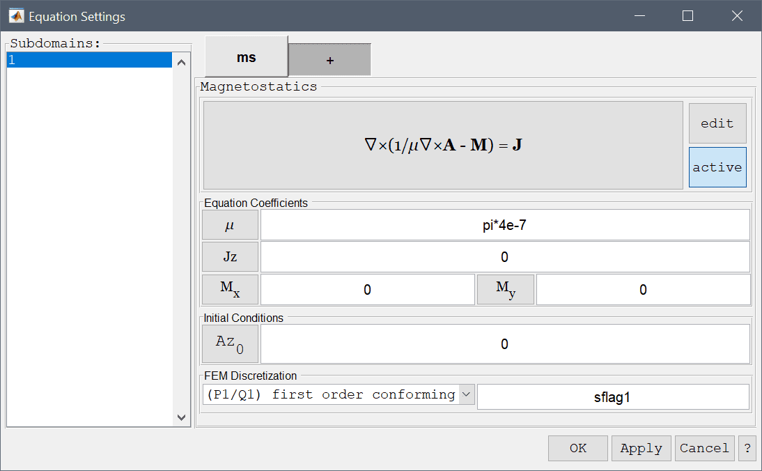
The magnetostatics physics mode models simplified Maxwell's equations and in two dimensions solves
\[ -\nabla\cdot( \frac{1}{\mu}\nabla A_z - \mathbf{M} ) = J_z \]
for the magnetic vector potential \(A_z\) in the z-direction where \(\epsilon\) is the permeability, \(\mathbf{M}\) the magnetization vector, and \(J_z\) the current density. In three dimensions the equations are simplified to exclude currents which reduces them to solving for a scalar magnetic potential \(V_m\)
\[ -\nabla\cdot( \mu\nabla V_m - \mu\mathbf{M} ) = 0 \]
In the Equation Settings dialog box shown below the equation coefficients, initial value for the magnetic potential can be specified. The FEM shape function space can also be selected from the drop-down combobox (1st through 5th order conforming P1/Q1 shape functions), or further specified in the corresponding edit field.
The magnetostatics physics mode features four boundary conditions, one prescribing the magnetic potential at a boundary, one for magnetic insulation zero potential, surface current, and magnetic insulation/symmetry. These boundary conditions are summarized in the table below
| Boundary Condition | Definition | Boundary Coefficient |
|---|---|---|
| Magnetic potential | Prescribed magnetic potential, \(A_z/V_m = A_{z,0}/V_{m,0}\) | Az0/Vm0 |
| Magnetic insulation/antisymmetry | Zero magnetic potential, \(A_z/V_m = 0\) | |
| Surface current | Prescribed current flow (flux), \(-\mathbf{n}\cdot (\frac{1}{\mu}\nabla A_z - \mathbf{M}/\mu\nabla V_m - \mu\mathbf{M}) = \mathbf{J}_s\) | Jx/y/z,s |
| Electric insulation/symmetry | Zero current flow (flux), \(-\mathbf{n}\cdot (\frac{1}{\mu}\nabla A_z - \mathbf{M}/\mu\nabla V_m - \mu\mathbf{M}) = 0\) |
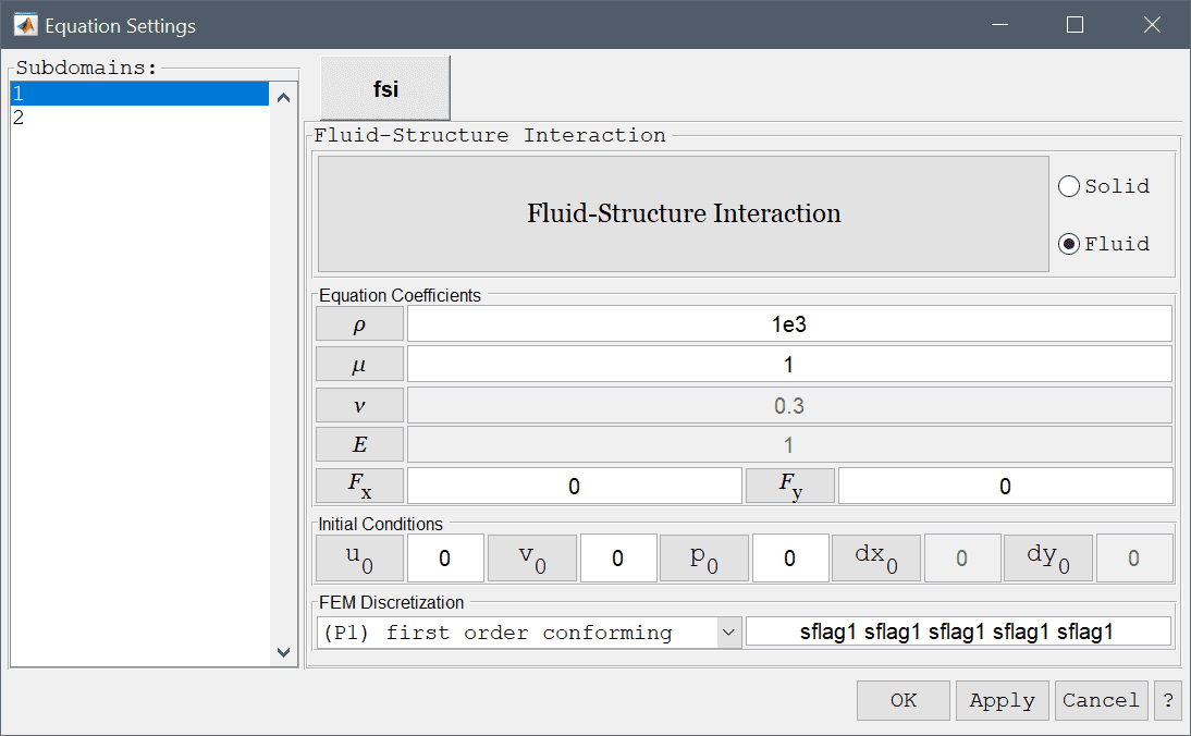
The Fluid-Structure interaction (FSI) physics mode supports modeling and simulation of how laminar fluid flows and solid materials interact. The flow field is governed by the Navier-Stokes equations
\[ \left\{\begin{aligned} \rho\frac{\partial\mathbf{u}}{\partial t} - \nabla\cdot(\mu(\nabla\mathbf{u}+\nabla\mathbf{u}^T)) + \frac{\mu}{\kappa}\mathbf{u} + \nabla p &= \mathbf{F} \\ \nabla\cdot\mathbf{u} &= 0 \end{aligned}\right. \]
for the velocity field \(\mathbf{u}\) and pressure \(p\). While the solid is modeled by the equilibrium equation
\[ -\nabla\cdot\mathbf{\sigma} = \mathbf{F} \]
where the constitutive law \(\mathbf{\sigma} = \mathbf{\sigma}(E)\) follows the Saint Venant-Kirchoff nonlinear material model for hyperelasticity.
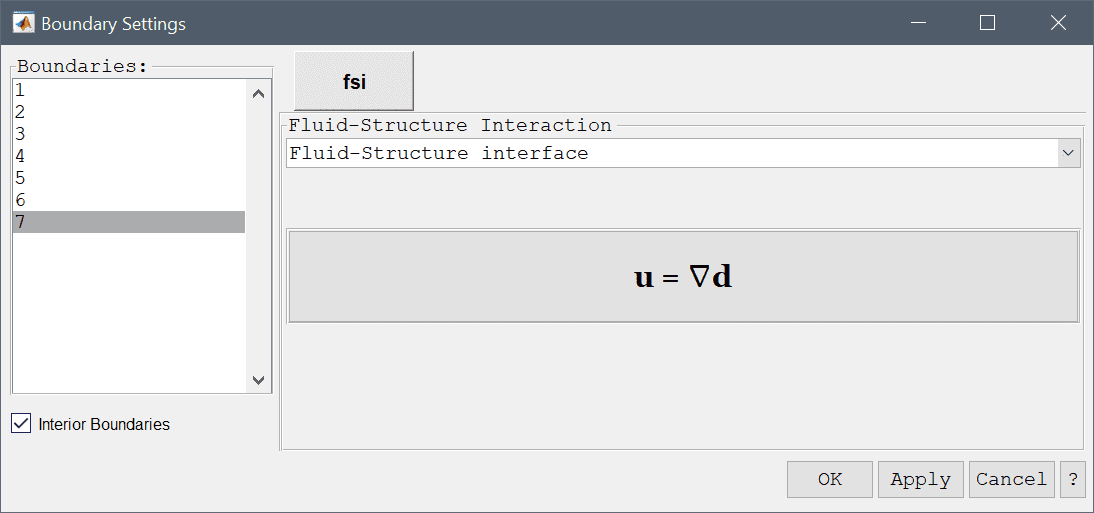
The fluid-structure interaction physics mode selection requires at least one Fluid and one Solid subdomain which can be selected with the labled radio buttons in the Subdomain Settings dialog box. This also enables/disables the corresponding equations coefficients density \(\rho\) and viscosity \(\mu\) for fluid domains, and density \(\rho\), Poisson's ratio \(\nu\), and modulus of elasticity \(E\) for solid domains.
Fluid domains allow for the same boundary conditions as for the Navier-Stokes physics mode, and on boundaries of solid domains prescribed displacements can be applied (using zero displacements to completely fix a boundary). Interior boundaries should be enabled with the corresponding check-box. Specifically, interior boundaries which are shared between fluid and solid domains should be prescribed with the Fluid-Structure interface condition to ensure that the interactions between the two domains are treated correctly.
| Boundary Condition | Definition | Boundary Coefficient |
|---|---|---|
| Wall/no-slip | Zero velocity, \(\mathbf{u} = 0\) | |
| Inlet/velocity | Prescribed velocity, \(\mathbf{u} = (u_0, v_0, w_0)\) | u0, v0, w0 |
| Neutral outflow/stress boundary | Zero stress, \(-\mathbf{n}\cdot (-p\mathbf{I} + \mu(\nabla\mathbf{u}+\nabla\mathbf{u}^T)) = 0\) | |
| Outflow/pressure | Prescribed pressure, \(p = p_0\) | p0 |
| Symmetry/slip | Zero normal velocity, \(\mathbf{n}\cdot\mathbf{u} = 0\) | |
| Prescribed displacement | Prescribed displacements, \(d_i = d_{i,0}\) | di,0 |
| Fluid-Structure interface | Fluid-structure interface boundary coupling |
Fluid-Structure interaction problems require a special solver to account for the mesh deformation and does not support coupling with other physics modes (see the corresponding Fluid-Structure Interaction (FSI) Solver section).
The Poisson equation physics mode solves the classic elliptic Poisson equation for the scalar dependent variable \(u\)
\[ d_{ts}\frac{\partial u}{\partial t} + \nabla\cdot(-D\nabla u) = f \]
where \(d_{ts}\) is a time scaling coefficient, \(D\) is a diffusion coefficient, and \(f\) is a scalar source term. In the Poisson Equation Settings dialog box shown below these equation coefficients, initial value \(u_0 = u(t=0)\) can be specified. The FEM shape function space can also be selected from the drop-down combobox (1st through 5th order conforming P1/Q1 shape functions), or further specified in the corresponding edit field.

The physics mode allows for both Dirichlet and Neumann (flux) boundary conditions. Dirichlet conditions prescribe a fixed value \(r\) of the dependent variable \(u = r\) on a boundary segment, while a Neumann condition will prescribe the normal flux to a boundary segment, that is \(-\mathbf{n}\cdot D\nabla u = g\), where \(\mathbf{n}\) is the outward directed normal, and \(g\) therefore represents the value of the inward directed flux. The available boundary conditions are summarized in the table below
| Boundary Condition | Definition | Boundary Coefficient |
|---|---|---|
| Dirichlet | Prescribed value, \(u = r\) | r |
| Neumann | Prescribed flux, \(-\mathbf{n}\cdot D\nabla u = g\) | g |
User defined equations can be prescribed by using the custom equation physics mode.
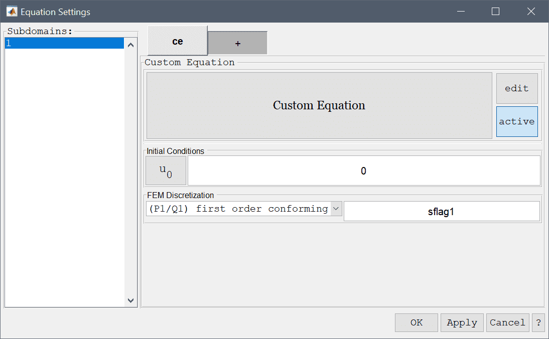
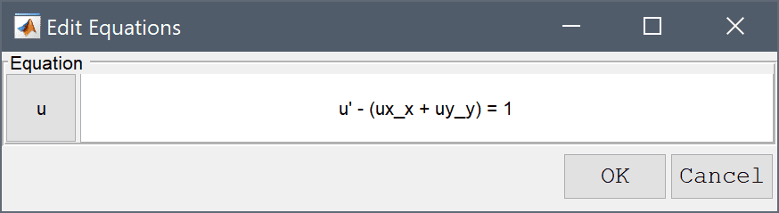
The equation specification can be accessed by either pressing the edit button next to the equation description, or the equation description itself. A dialog box will appear showing one edit field for equation and corresponding dependent variable.
Boundary conditions are specified similar to the Poisson equation described above.
Note that the other physics mode equations are defined similarly and can also be edited by pressing the edit button in the corresponding tabs of the equation settings dialog box.
The syntax for equation specifications tries to as close as possible look like how one would write a partial differential equation with pen and paper. If for example the dependent variable is u like in the example above, then u' corresponds to the time derivative, ux the derivative in the x-direction, ux_x a second order derivative in the x-direction (to which partial integration will be applied according to the standard finite element derivation of the weak formulation), and u_t is the variable u multiplied with the fem test function, thus it will be assembled to the iteration matrix instead of the right hand side. The following table describes the syntax and legal operators
| Syntax | Description | Formula |
|---|---|---|
| u | Dependent variable name | \(u\) |
| x | Space dimension name | \(x\) |
| ux | Derivative in x-direction, rhs | \(\frac{\partial u}{\partial x}\) |
| u_t | Dep. var multiplied with test function | \(u\cdot v\) |
| u_x | Derivative of test function | \(u\cdot \frac{\partial v}{\partial x}\) |
| ux_t | Derivative in x-direction | \(\frac{\partial u}{\partial x}\cdot v\) |
| ux_x | 2nd derivative in x-direction | \(\frac{\partial u}{\partial x}\cdot\frac{\partial v}{\partial x}\) |
| uxx_x | 3rd derivative in x-direction | \(\frac{\partial^2 u}{\partial x^2}\cdot\frac{\partial v}{\partial x}\) |
| ux_xx | 3rd derivative in x-direction | \(\frac{\partial u}{\partial x}\cdot\frac{\partial^2 v}{\partial x^2}\) |
| uxx_xx | 4th derivative in x-direction | \(\frac{\partial^2 u}{\partial x^2}\cdot\frac{\partial^2 v}{\partial x^2}\) |
| + | Addition | |
| - | Subtraction | |
| * | Multiplication | |
| / | Division | |
| sqrt() | Square root | |
| Power | ||
| () | Delimit by enclosing in parentheses |
where v is a test function. The equation syntax parser accepts numeric constants and coefficients defined in the fea.coef field. Higher dimensions work analogously and the space dimension x can be substituted with the others arbitrarily. For a more complicated example look at Black-Scholes Equation in the tutorials section.
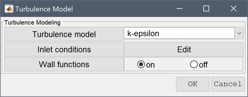
Turbulence models are available for flow physics modes and can be used to simulate flows with unresolved turbulent effects. The Turbulence Model dialog box allows for selecting the turbulence model, as well as using turbulent Wall functions and prescribing turbulent quantities on Inlet conditions boundaries (only used by the OpenFOAM external CFD solver).
The different available models depends on the solver which is be used (FEATool built-in, OpenFOAM, or SU2) according to the following table
| Turbulence Model | FEATool (Built-in) | OpenFOAM | SU2 |
|---|---|---|---|
| Laminar | x | x | x |
| Algebraic | x | ||
| Spalart-Allmaras | x | x | |
| k-epsilon | x | ||
| k-epsilon (RNG) | x | ||
| k-epsilon (realizable) | x | ||
| k-omega | x | ||
| k-omega (SST) | x | x |
The algebraic turbulence model available in FEATool is based on Prandtl's mixing length theory, and works by introducing an additional turbulent viscosity in regions where velocity fluctuations are expected to be high [1]. That is
\[ \mu_{E}(\mathbf{x}) = \mu_F + \mu_T(\mathbf{x}) \]
where the total or effective viscosity \(\mu_{E}\) is the sum of the viscosity of the fluid \(\mu_F\) and the turbulent viscosity \(\mu_T\). This lowers the local Reynolds number allowing the equations to converge.
By using dimensional analysis the kinematic turbulent viscosity must be the product of a velocity scale and a length scale. Moreover, assuming that the small scale turbulent velocity fluctuations (Reynolds stresses) to be modeled can be related to the mean velocity, then we have that the turbulent viscosity can be expressed as
\[ \mu_T(\mathbf{x}) = \rho\ l_{mix}(\mathbf{x})^2|\nabla u| \]
where the mixing length \(l_{mix}\) represents the average length a turbulent fluid packet and eddy can travel before breaking up. This can be modeled as the minimum of the shortest distance to the walls, and a characteristic length \(l_c\), that is
\[ l_{mix} = min(\kappa\ l_{wall}, Const\ l_c) \]
where \(\kappa = 0.41\) is the von Karman constant. This model assumption works well for simple two-dimensional flows such as for example in wakes, jets, and mixing, shear, and boundary layers. Modeling constants and characteristic lengths for these types of flow regimes have been determined empirically, and are given in the table below [2], where the constant 0.09 is used by FEATool to compute the turbulent mixing length.
| Flow type | \(Const\) | \(l_c\) |
|---|---|---|
| Mixing layer | 0.07 | Layer width |
| Jet | 0.09 | Jet half-width |
| Wake | 0.16 | Wake half-width |
| Axisymmetric jet | 0.075 | Jet half-width |
| Boundary layer (outer) | 0.09 | Boundary layer thickness |
Note that this model is not really accurate or recommended for complex flows such as those involving separation and/or recirculation.
References:
[1] Versteeg HK, Malalasekera W. An Introduction to Computational Fluid Dynamics: The Finite Volume Method. Longman Scientific and Technical, England, 1995.
[2] Rodi W. Turbulence Models and their Application in Hydraulics, IAHR, Netherlands, June, 1980.
For models with strong and dominating flow and convective effects such as often found in convection-diffusion, heat transfer, and fluid dynamics problems, it often happens that solvers have difficulty converging, especially if the grid sizes are too coarse. In this case one can employ artificial stabilization techniques, essentially adding "smart" artificial and numerical mesh dependent diffusion, to assist with solver convergence.
The Artificial Stabilization dialog box allows control of isotropic artificial diffusion, anisotropic streamline diffusion, shock-capturing, and pressure stabilization and constraint options. Turning coefficients are also provided to control the strength of the introduced artificial and numerical diffusion.
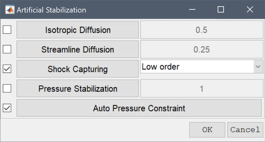
The Isotropic Diffusion option when enabled, adds artificial diffusion of magnitude delta_ad*h_grid*|u| in all directions, where delta_ad is the tuning coefficient, h_grid the local mean diameter of grid cells, and |u| the magnitude of the convective velocity field. This is a robust but very diffusive stabilization option.
Streamline Diffusion, alternatively modifies the finite element test function space to only add a stabilization coefficient of the form delta_sd*h_grid/|u| in the direction of the flow, so as to minimize artificial diffusion in (cross) directions not required.
Shock Capturing optionally adds non-linear (FEM-TVD) stabilization to minimize unphysical over and undershoots due to convection, that is shocks (which can be present for example during for example supersonic flows). This renders all stabilized equations nonlinear but should be the most accurate form of stabilization, especially where shocks and steep gradients are present in the flow. Shock capturing can be selected between low order (more diffusive and stable) and high order (least diffusive and most accurate).
Pressure Stabilization (PSPG) is not convective stabilization, but necessary and automatically enabled for FEM discretizations where all dependent variables use 1st order (P1) discretizations (but not required for traditional P2P1 discretizations). A tuning coefficient is also present to allow for tuning of the artificial stabilization.
Auto Pressure Constraint automatically adds an integral constraint to the pressure (zero mean pressure) if no boundary conditions on the pressure are present (no outflows), as otherwise the pressure level is undetermined for incompressible flows, leading to difficulties for FEM solvers to converge.