|
|
FEATool Multiphysics
v1.18.0
Finite Element Analysis Toolbox
|
|
|
FEATool Multiphysics
v1.18.0
Finite Element Analysis Toolbox
|
The last step in the simulation process is postprocessing and visualization. FEATool automatically switches to postprocessing mode after a solution has been computed. Alternatively, one can press the ![]() mode button to manually switch to postprocessing mode.
mode button to manually switch to postprocessing mode.
The ![]() toolbar button and corresponding menu option opens the Postprocessing Settings dialog box which controls various postprocessing options explained in the section below.
toolbar button and corresponding menu option opens the Postprocessing Settings dialog box which controls various postprocessing options explained in the section below.
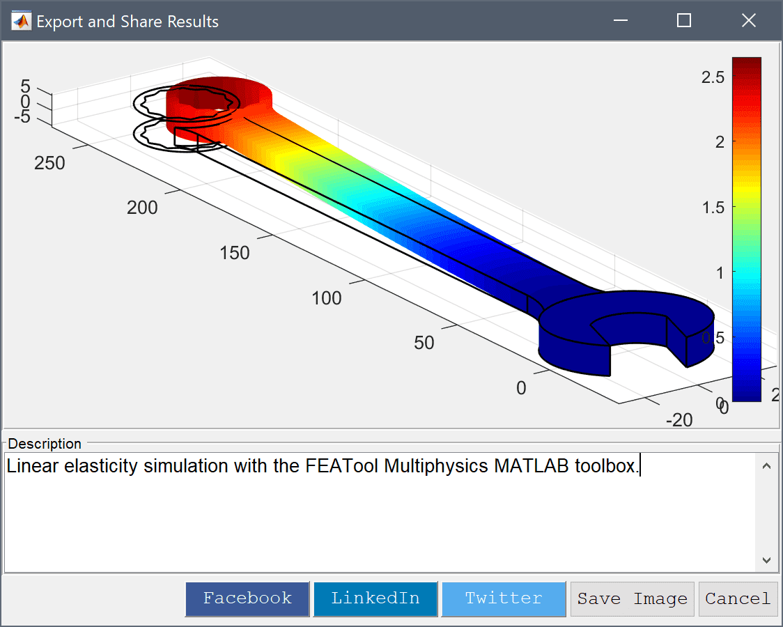
Images or snapshots of the current plot can be exported and saved in jpeg or png formats by using the ![]() toolbar button. In the corresponding dialog box exporting and sharing results to Facebook, LinkedIn, and Twitter is also supported.
toolbar button. In the corresponding dialog box exporting and sharing results to Facebook, LinkedIn, and Twitter is also supported.
The ![]() and
and ![]() buttons allow exporting the currently visualized postprocessing data as ParaView Glance (VTP) and Plotly web plots, respectively. These types of web plots can be conveniently be inspected, manipulated, exported, and shared via the web. An internet connection may be required to access and download the corresponding web reader, and the exported plot data might be required to be loaded into the viewer manually.
buttons allow exporting the currently visualized postprocessing data as ParaView Glance (VTP) and Plotly web plots, respectively. These types of web plots can be conveniently be inspected, manipulated, exported, and shared via the web. An internet connection may be required to access and download the corresponding web reader, and the exported plot data might be required to be loaded into the viewer manually.
The Post menu allows for switching to Postprocessing Mode, opening the Postprocessing Settings... dialog box, and advanced postprocessing options such as subdomain and boundary integration, and export and interfacing with external tools as explained in the section below.
The visualization options in Postprocessing Settings dialog box shown in the following figure include choosing pre-defined or entering user defined custom expressions for surface, height, contour, slice, arrow, and deformation plots. Moreover, there are options for choosing the solution to display (for time dependent solutions), selecting or excluding which cells to display, and setting the min and max plot scale limits, and switching the colorbar on and off. The postprocessing options are explained in more detail below.
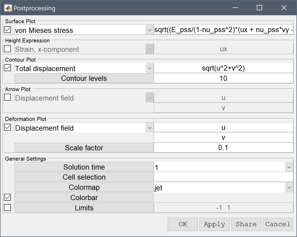
Note that as is usual in FEATool postprocessing expressions accept general expressions involving dependent variables, space dimensions, constants, and mathematical operators. Complex expressions such as v+ux+sin(2*pi*y) where u and v are dependent variables (so that ux is the derivative in the x-direction), are perfectly valid.
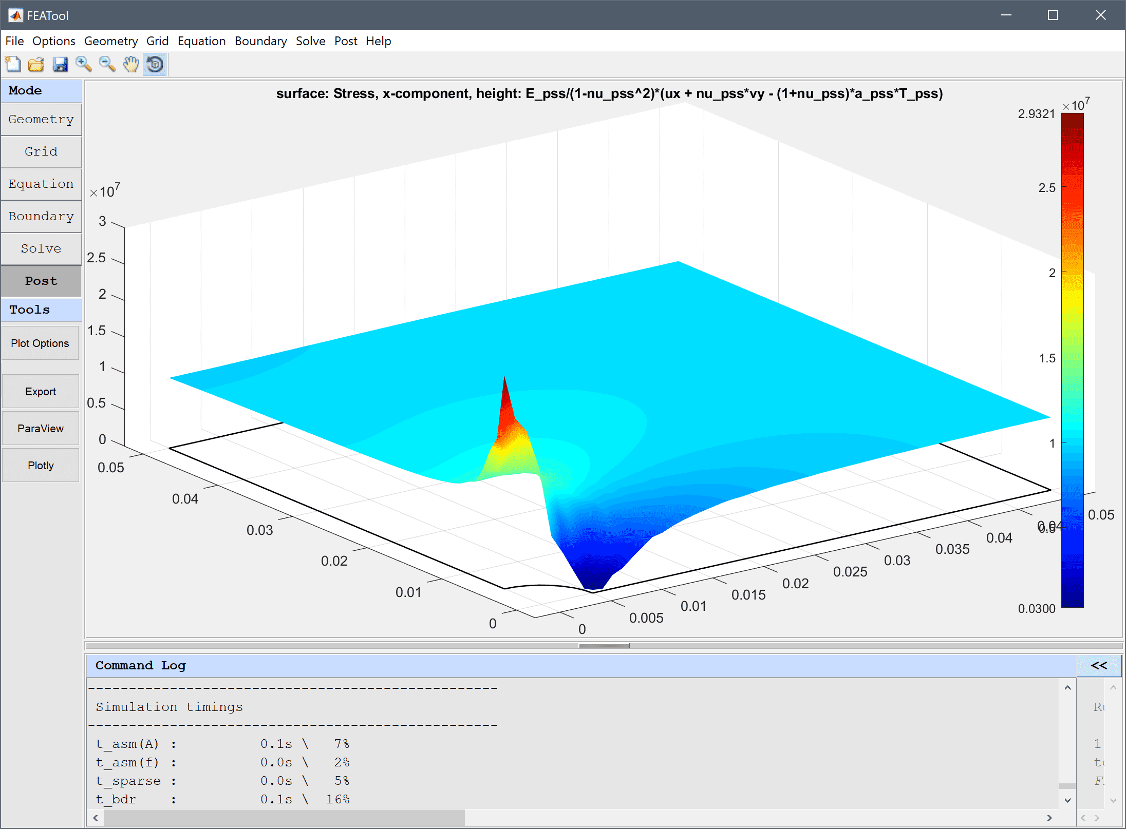
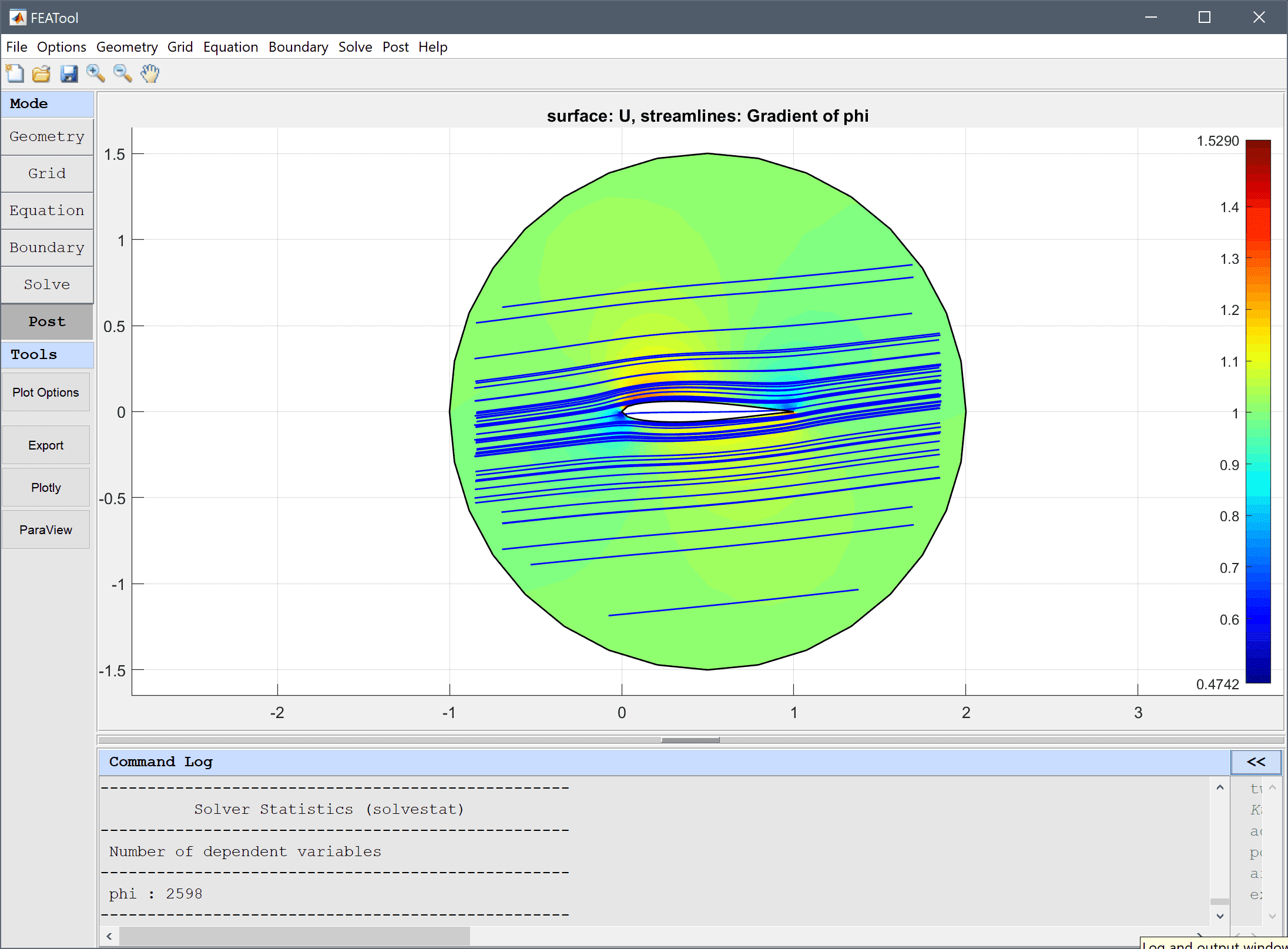
Surface plots allows visualization of both predefined postprocessing expressions and user defined ones on the domain surface. To use the surface plot option mark the corresponding check box and enter the expression to visualize. If desired one can change the colormap of the surface plot.
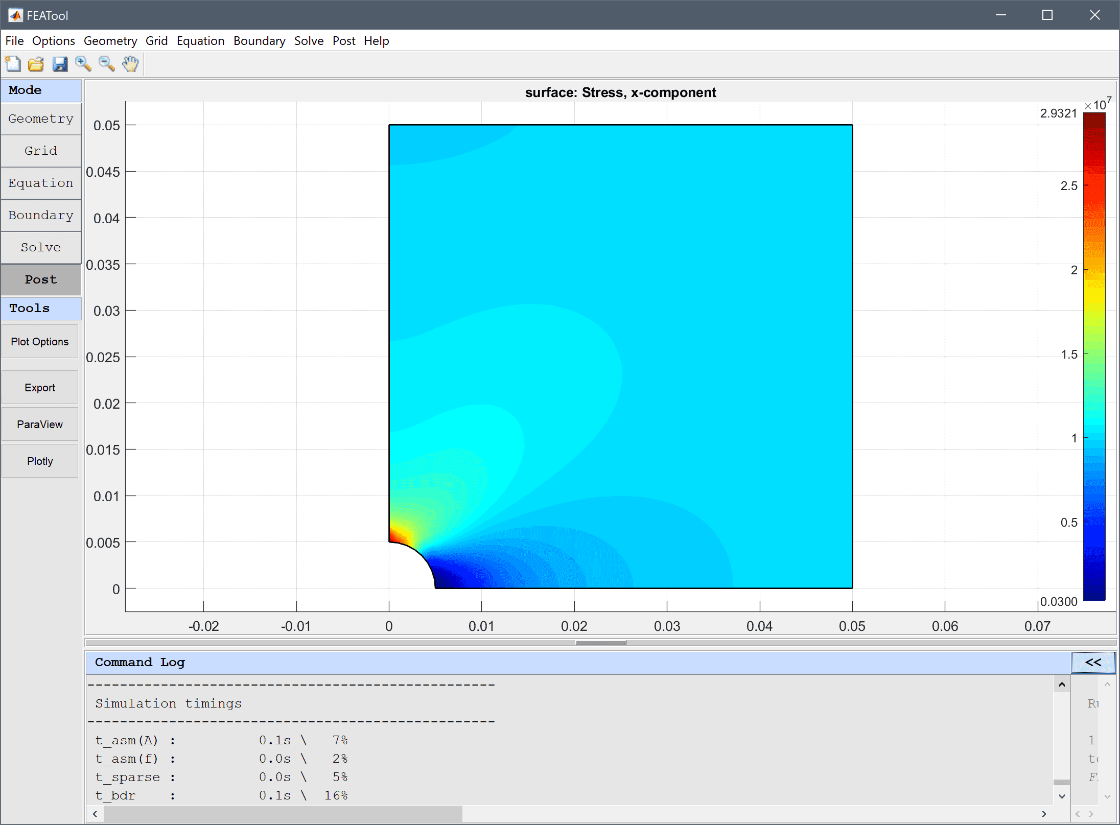
For convenience, clicking on a 2D surface plot will evaluate the surface expression at the corresponding point and print the evaluated value.
In two dimensions the height expression option is available which scales a surface plot in the z-direction with the computed value of the height expression. To use the height expression option check the corresponding check box.
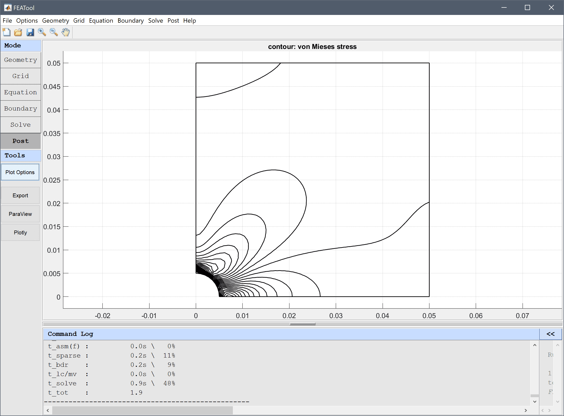
Two dimensional problems also allow for contour or isoline plots. To use the contour plot option mark the corresponding check box and select or enter an expression for the contour values. The contour values can be specified in the Contour levels edit field, either as an integer for the number of contours, or a space separated vector to specify fixed values for the contour levels. If desired one can also change the colormap of the contour plot.
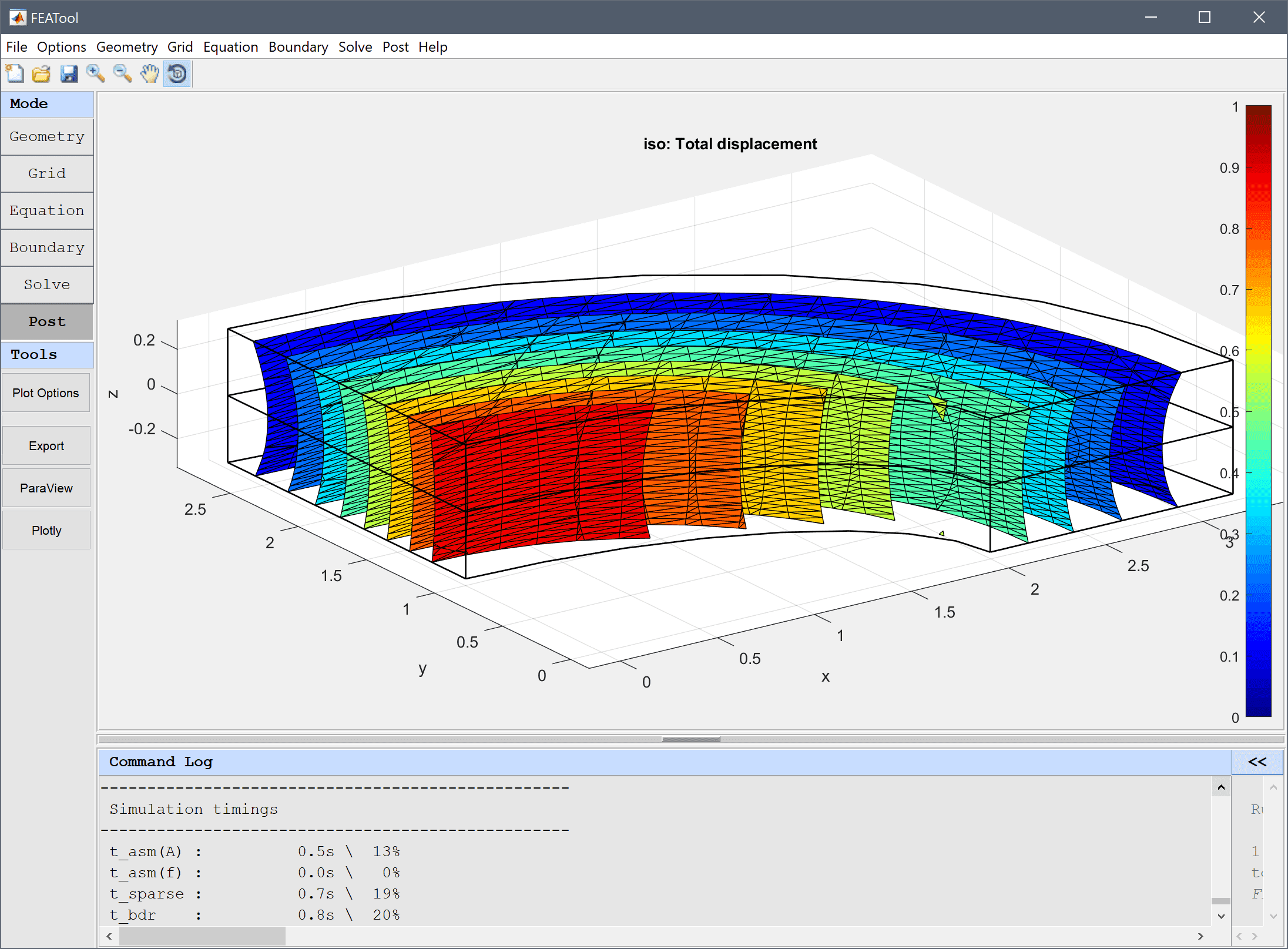
Similarly to contour plots, three dimensional problems allow for isosurface plots. To use the isosurface plot option check the corresponding check box and select or enter an expression for the isosurface values. The iso plot values can be specified in the Iso levels edit field, either as an integer for the number of isosurfaces, or a space separated vector to specify fixed values for the iso levels. If desired one can also change the colormap of the iso-surface plot.
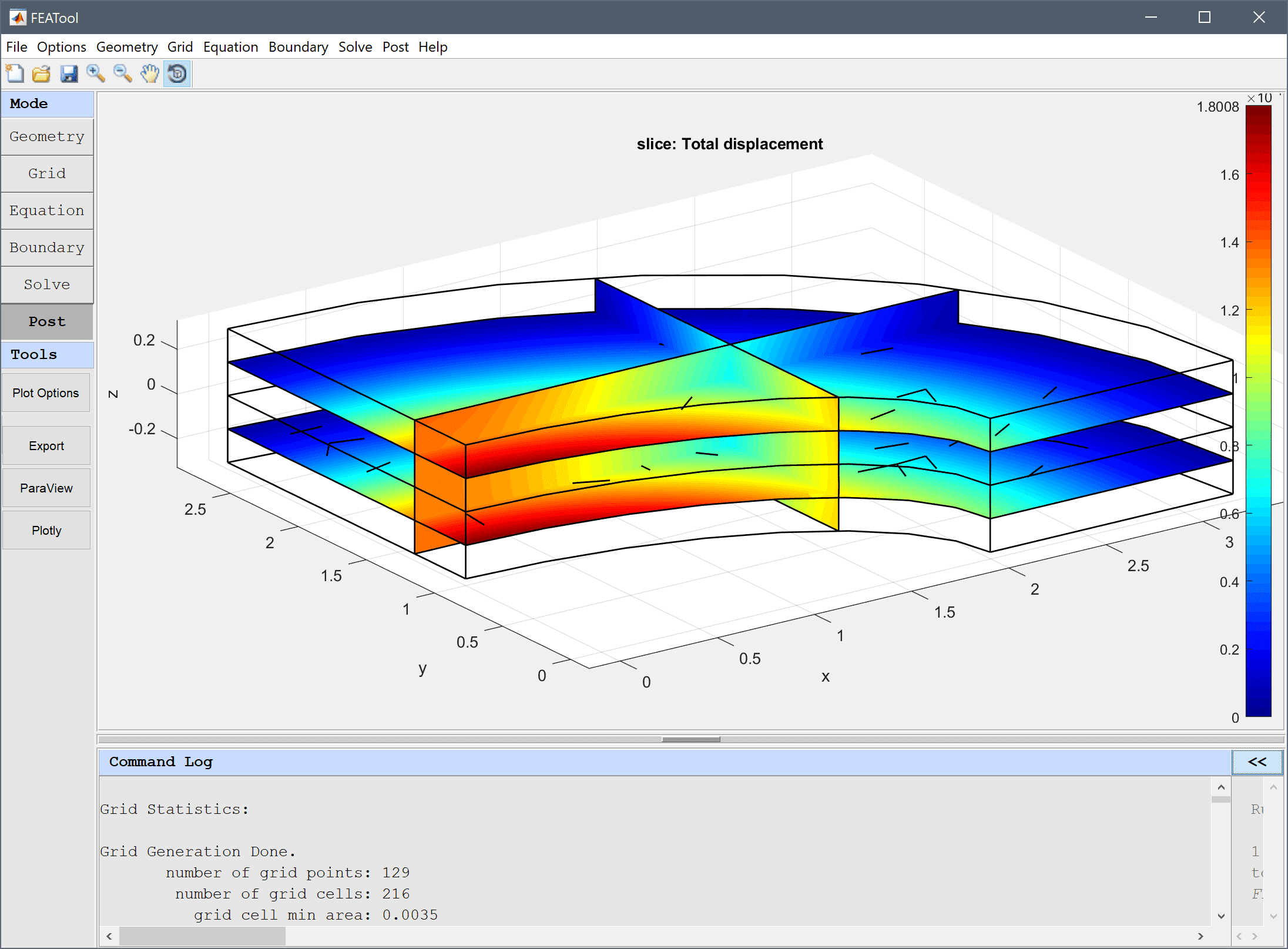
Three dimensional problems also allow for slice plots which are surface plots perpendicular to the coordinate axes. To use the slice plot option mark the corresponding check box and select or enter a slice expression. The Slice positions can be prescribed as a single integer signifying the number of equally spaced slices, or a space separated list indicating the exact position of each slice for the chosen axis.
Arrow plots are available in two and three dimensions. To use arrow plots mark the corresponding check box and select or enter expressions for the vector field defining the direction of the arrows. One can also enter a scaling factor for the arrows and select the arrow colors.
Streamline plots are also available in two and three dimensions. To plot streamlines mark the corresponding check box and select or enter expressions for the vector field defining the streamlines. One can also select the number of streamlines and the color.
Deformation plots are available in two and three dimensions and deforms the geometry and surface related plots correspondingly. To use the deformation plot, mark the corresponding check box and select or enter expressions for the vector field defining the direction of the deformation. The deformation scale factor allows for tuning of the deformation scale in relation to the geometry size.
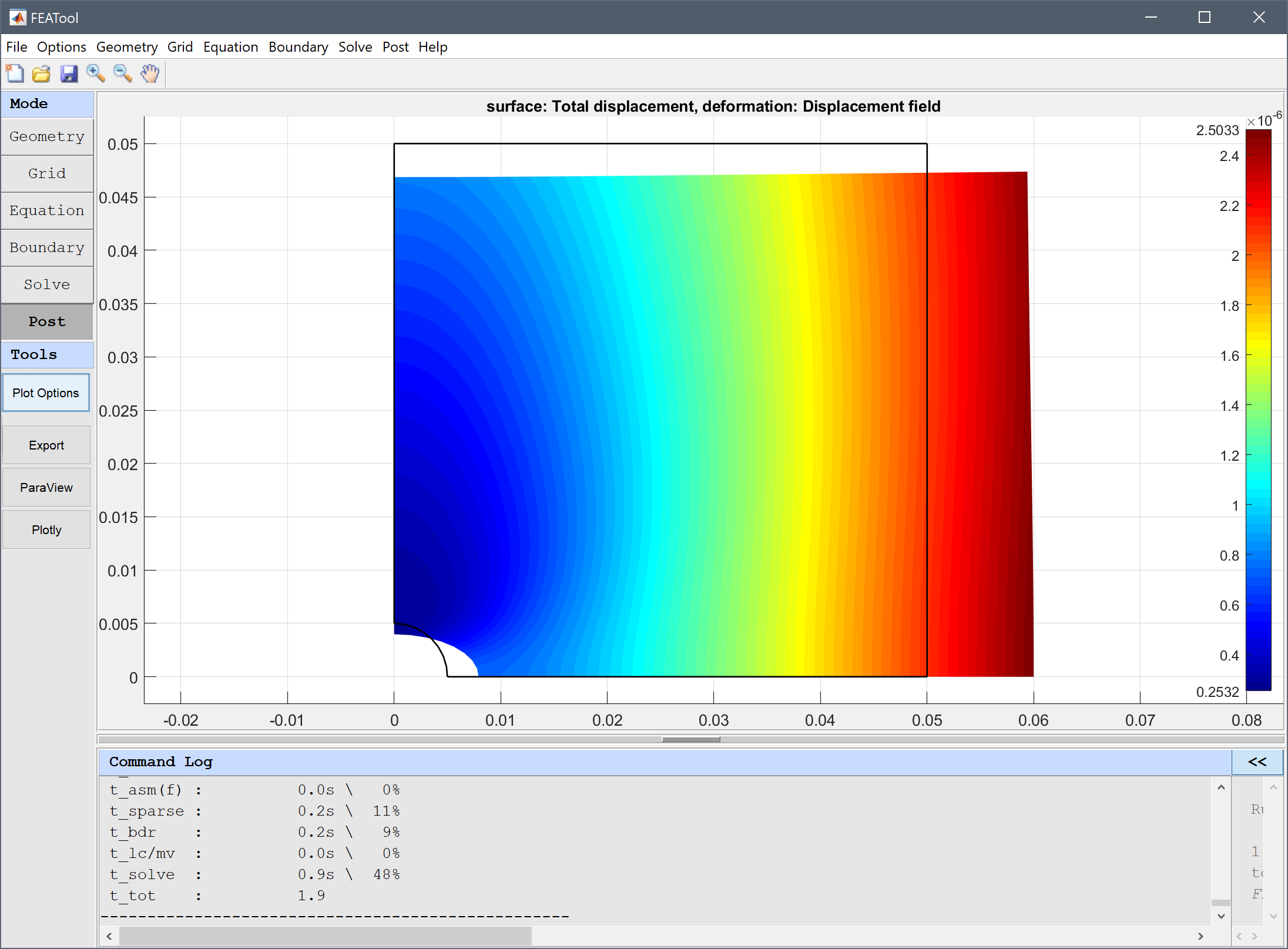
General settings allow for selecting Solution time (or Eigenvalue/frequency for eigenvalue problems) if several solutions are available as with time-dependent problems. Moreover, with Cell selection one can limit the postprocessing to a certain subset of cells by entering a logical expression. For example, the cell selection expression x>0 would only plot cells on the positive x-axis. Colormap selects a colormap to use, the Colorbar check box toggles the colorbar on and off, and the Limits vector indicates and prescribes the minimum and maximum values of the colorbar range. In 3D a Transparency slider is also available to control the opacity of the plots.
The Post menu allows for the following advanced postprocessing options.
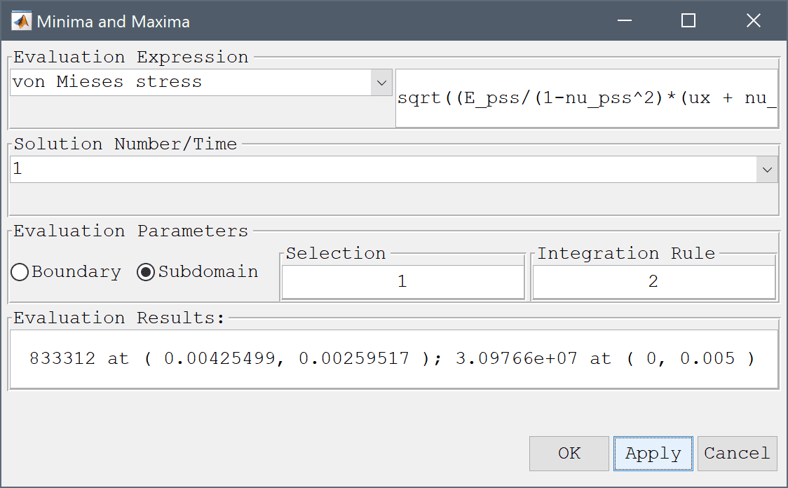
Evaluates the minimum and maximum values for expressions on subdomains (minmaxsubd) or boundaries (minmaxbdr). The Evaluation Expression can either be selected from a list of predefined postprocessing expressions, or entered as a user defined custom expression in the corresponding edit field. The Solution Number/Time can also be selected if more than one is present. In the Selection edit field a space separated list of Subdomains or Boundaries is specified for which the minima and maximia should be evaluated. The numerical Integration Rule prescribes how many evaluation points should be used for each grid cell in the evaluation process. The result will be printed in the Evaluation Result field as well as the command log in the main GUI.
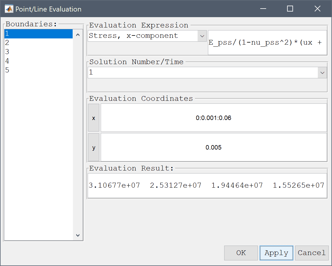
Allows both pre and user-defined expressions to be evaluated at single points or lines (evalexpr). Coordinates for the evaluation points can be entered as space separated vectors for each space dimension in the corresponding edit fields. The Solution Number/Time to evaluate can be selected in the drop-down listbox. The result will be printed in the Evaluation Result field as well as the command log in the main GUI. By selecting one or more of the Boundaries in the left hand side listbox, evaluation points at the boundaries will automatically be used.
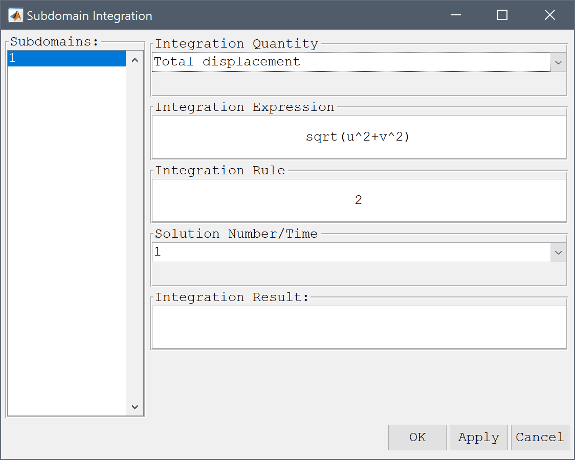
Integration of postprocessing expressions over subdomains Subdomain Integration... (intsubd) and boundaries Boundary Integration... (intbdr) can be performed by selecting the corresponding menu options. The integration dialog box allows for selecting predefined postprocessing or entering user defined expressions in the Integration Expression edit field. Numerical Integration Rule, Solution Number/Time, and Subdomain/Boundary: to integrate over can also be set. The result will be printed in the Integration Result field as well as the command log in the main GUI.
The Slice Plot... menu option allows for plotting and visualization of 3D slices onto a 2D plane. When selected, the Slice Plot Settings dialog box is opened where one must first specify a slicing plane via a Plane point and Plane normal. After selecting from the 2D plot options and pressing OK or Apply a new figure will open with the projected slice plot (a preview of the slice is also shown in the 3D plot axis).
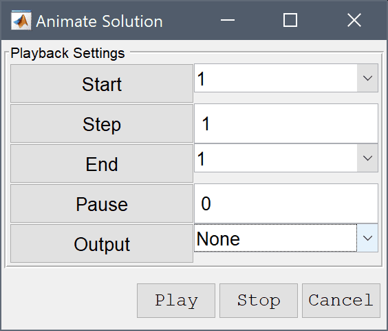
Animations of the results (postanimate) can be created by selecting the Animate button in the Postprocessing Settings dialog box or Animate/Playback Solution... from the Post menu. The Animate Solution dialog box allow for selecting start/end solutions (time), the step factor (number of solutions to skip between each frame), a pause (in seconds) between each frame, and optionally an image or movie file format to record/save to (JPEG, PNG, MP4, AVI). Pressing the Play / Stop buttons starts and stops the playback and recording process, respectively.
Simulation and postprocessing data can be exported to CSV, Excel (xlsx), and ParaView (VTK) and (VTP) formats, as well as Webbrowser compatible files (html).
To export data first select a corresponding Post > Export Data... menu option in the in the toolbox GUI. In the Data Export dialog box enter a space separated list of expressions to evaluate and export (see the section on coefficient and expressions for a description of valid postprocessing expressions). By default, this is populated with the current visible postprocessing expressions. For time dependent simulations, a solution time for which the expressions will be evaluated can also be selected. Evaluation coordinates/points are set to the grid vertices by default, but can be changed for CSV and Excel formats to evaluate in any points. Pressing the Export button will prompt to choose a file name to export, corresponding to the selected csv, xlsx (Excel), vtk, and vtp file formats.
To export data manually one can also make use of the evalexpr and evalexprp functions and the MATLAB Command Line Interface (CLI). To do this, first export the problem struct from the GUI to the main MATLAB workspace by selecting Export > FEA Problem Struct To Main Workspace from the File menu. Then call evalexpr to create a temporary variable with data to export.
For example to evaluate and export the coordinates x, y, dependent variable u, gradient in the x-direction ux, and the evaluated expression 2*sin(u*x)^2 in the grid points p the following m-file script can be used
% Cell array of expressions to evaluate.
c_data = { 'x', 'y', 'u', 'ux', '2*sin(u*x)^2' };

% Coordinates of evaluation points.
p = fea.grid.p;

% Evaluate expressions and store results in data array.
data = zeros( size(p,2), length(c_data) );
for i=1:length(c_data)
  data(:,i) = evalexpr( c_data{i}, p, fea );
end
The data can now be saved and exported to a file with the save, csvwrite, or fprintf commands in various formats, for example the command
save( '-ascii', 'mydata.txt', 'data' )
saves the data array to the text file mydata.txt.
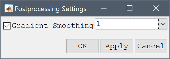
Selecting the advanced Postprocessing Settings... from the Post menu opens a dialog box where the settings for smoothing of derivatives of dependent variables can be modified. The checkbox toggles gradient smoothing on and off for surface type plots. As gradient smoothing can be quite expensive (and also not required) for problems higher order discretizations, one can also select a cutoff order from where smoothing will not be used (default used only on 1:st order discretization schemes).
More advanced and customized postprocessing and visualization can be performed on the MATLAB command line interface (CLI) and with MATLAB scripts. The fea model data can either be exported from the FEATool GUI by selecting the Export Model Data Struct to MATLAB option from the File menu, or computed or loaded directly from an m-file model script.
In addition to the custom FEATool postprocessing functions listed below, all standard MATLAB functions and toolboxes can be used to process model data. Below is a list of examples using CLI postprocessing functionality.
The following functions can be used on the command line for postprocessing and visualization.
| Function | Description |
|---|---|
| export_csv | Export CSV postprocessing data |
| export_xls | Export postprocessing data to Excel |
| evalexpr | Evaluate expressions in given points |
| evalexprp | Evaluate expressions in grid points |
| impexp_vtk | Export ParaView VTK data format |
| impexp_vtp | Export ParaView VTP data format |
| intbdr | Integrate expression on boundaries |
| intsubd | Integrate expression in subdomains |
| minmaxbdr | Evaluate minima and maxima on boundaries |
| minmaxsubd | Evaluate minima and maxima in subdomains |
| plotbdr | Plot and visualize boundaries |
| plotedg | Plot and visualize edges (3D) |
| plotsubd | Plot and visualize subdomains |
| postplot | Postprocessing and visualization function |
| postanimate | Create animations of results |
| postextrude | Extrude 2D fea data for 3D postprocessing |
| postrevolve | Revolve axisymmetric 2D fea data for 3D postprocessing |
| princse | Calculate principal stresses |