|
|
FEATool Multiphysics
v1.18.0
Finite Element Analysis Toolbox
|
|
|
FEATool Multiphysics
v1.18.0
Finite Element Analysis Toolbox
|
This section describes the different physics solvers available with the FEATool Multiphysics toolbox. Physics solvers compute numerical approximations to equations and boundary conditions with discretization schemes such as FDM/FEM/FVM. This results in sparse matrix systems which are subsequently solved (inverted) to yield discrete and approximate numerical solutions to the equations.
FEATool features integrated GUI and CLI interfaces to the linear and non-linear stationary (solvestat), time-dependent (solvetime), and eigenvalue (solveeig) multiphysics solvers. In addition, interfaces to external solvers, such as the Computational Fluid Dynamics (CFD) solvers OpenFOAM and SU2, and the FEA solver FEniCS is also built-in.
The external solver interfaces allow for setting up and defining multiphysics problems directly in MATLAB with the FEATool GUI and CLI interfaces, then export and solve them with the external solvers. Afterwards, the solutions can automatically be imported into the FEATool GUI for further post-processing. Moreover, the multi-simulation solver approach employed by FEATool conveniently allows switching between several solvers for the same problem with one-click, this can be very useful when comparing and validating results and solutions.
After geometry, grid, and equation and boundary conditions have been defined one can switch to solve mode by either pressing the ![]() mode button, or by selecting Solve Mode in the Solve menu. The solve mode toolbar buttons and menu actions are the following
mode button, or by selecting Solve Mode in the Solve menu. The solve mode toolbar buttons and menu actions are the following
The built-in solvers allow for solving coupled stationary, time-dependent, and eigenvalue/frequency multiphysics problems, for which solver settings and parameters and are discussed in the following.
The Solver Settings control panel and dialog box shown below can be opened by pressing the corresponding ![]() toolbar button or by selecting Solver Settings... in the Solve menu. The solver settings dialog box allow selecting and configuring the built-in multiphysics solvers.
toolbar button or by selecting Solver Settings... in the Solve menu. The solver settings dialog box allow selecting and configuring the built-in multiphysics solvers.
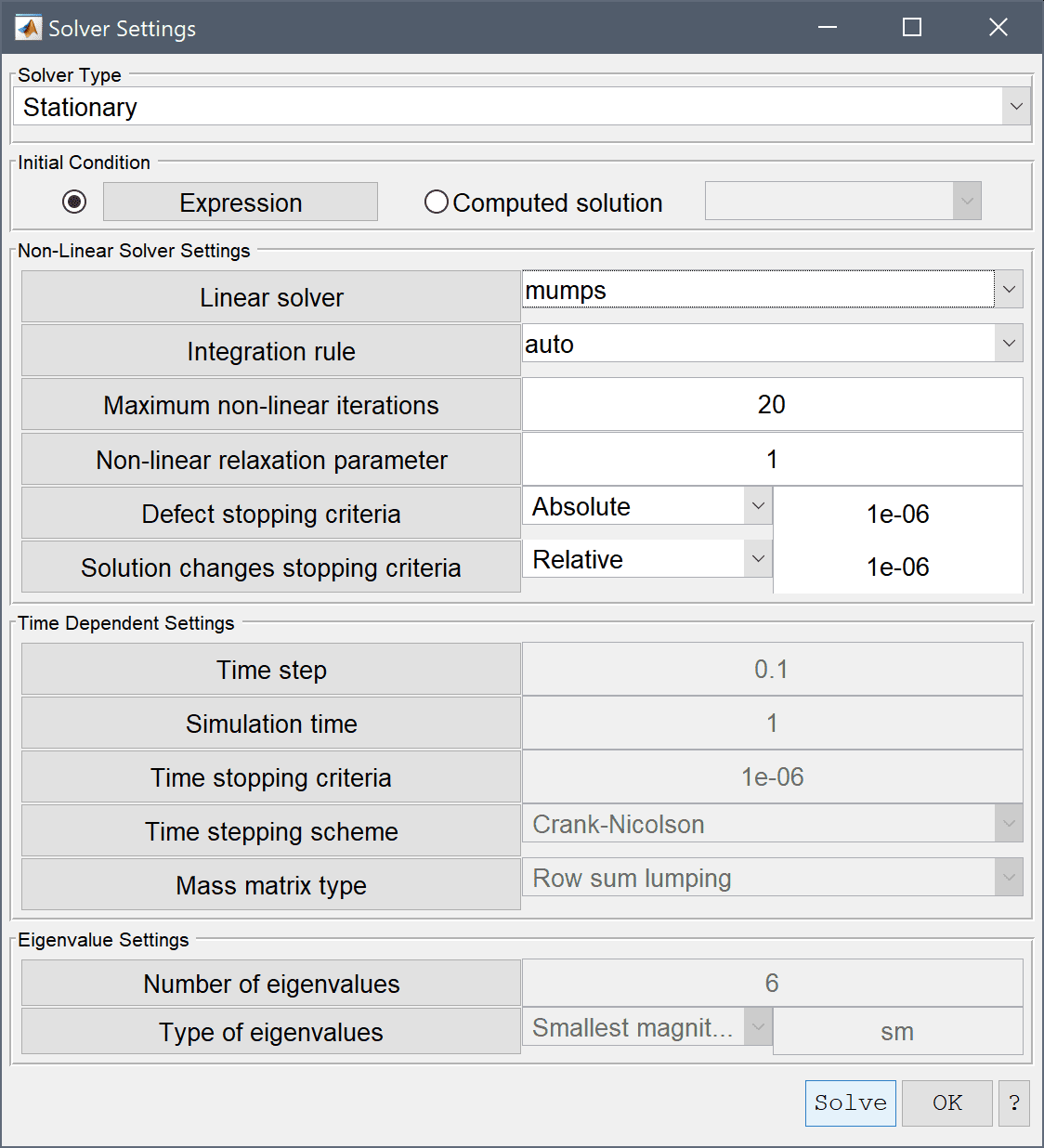
The Solver Type drop-down box allows for either of the
solvers to be selected. The built-in multiphysics solvers are monolithic, meaning that all equations and dependent variables are discretized and solved together in a large coupled system, rather than iteratively solving a segregated set of smaller decoupled systems. This typically allows for faster and more robust convergence behavior at the expense of higher memory usage.
The Initial Condition setting controls whether initial values should be computed from Expressions (from the equation settings initial value fields), or use a previously Computed solution. In the latter case the initial solution can be selected from the corresponding list box. Note that for this to work the geometry, grid, physics modes, and finite element shape functions must all remain the same.
The Linear solver used to solve sparse matrix systems can be selected from the following options
The default linear solver option is to use either the built-in direct solver (MATLAB's backslash operator) or, alternatively the direct solver mumps which can be noticeably faster and more efficient for many problems. Direct solvers are very robust and fast for a wide range of problems, but are not as memory efficient as iterative solvers such as gmres, bicgstab, or amg. The algebraic multigrid amg solver is experimental, but when it works it potentially can combine the best of solving speed with memory efficiency. Users can also incorporate their own or custom linear solvers by overloading or editing the solvelin function.
The Integration rule or numerical quadrature order used to numerically approximate equation integrals is automatically set to 1 + max(FEM shape function order) by default, but can also be set manually between 1st to 5th order if desired.
A fixed point/Newton non-linear solution process is automatically used when dependent variables are detected in equations and/or boundary coefficients. The Non-Linear Solver Settings allows control over the Maximum number of non-linear iterations, and the Non-linear relaxation parameter which is the fraction of the new to old solution to weigh in to the next non-linear iteration. The non-linear solver will terminate and stop when both the Defect stopping criteria and Solution changes stopping criteria are met which can be set to be measured in either absolute or relative error norms.
See the Non-linear Solver Strategy section below for strategies solving highly non-linear problems.
The Time Dependent Settings control time-stepping parameters when using a time-dependent solver. Time step sets the time step size for the time-stepping schemes. Time dependent simulations will terminate when either the accumulated time has reached the specified Simulation time, or the normed changes in the dependent solution variables are smaller than the Time stopping criteria, which would indicate a stationary state.
The Time stepping scheme setting allows choosing between the following schemes
The default Crank-Nicolson scheme works well in most situations, for very non-linear or sensitive time-stepping problems one can use the backward Euler method which is more robust but less accurate (to compensate smaller time steps can be used).
Lastly, one can choose between using the Full mass matrix, Row row-sum lumped (default), Diagonal lumped, or consistent HRZ-lumped Mass matrix type representations.
In the Eigenvalue Settings frame one can control the Number of eigenvalues to be computed, as well as the Type of eigenvalues to find (smallest/largest or a search region around a specified eigenvalue/frequency).
Solver hooks allow direct access to, and modification of, the finite element problem struct and matrices before and after linear solver calls in both the stationary (solvestat) and time-dependent (solvetime) solution processes. This enables implementation of non-standard equations and boundary conditions, such as for example periodic and non-axis aligned slip boundary conditions. Two classes of solver hook functions are available, general and boundary hooks.
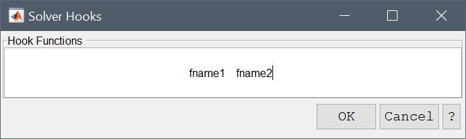
To define a general solver hook a function must first be created (here it is for example named fname, and a corresponding m-file function must exist in the MATLAB paths or current working directory). To be activated the function name must be entered in the "Solver Hooks" dialog box (which is opened when selecting Solver Hooks... in the Solve menu), which corresponds to the fea.sol.settings.hook field when modeling using the CLI and scripting interfaces instead of the GUI.
The solver hook function must have the following call signature
[ A, f, fea ] = fname( A, f, fea, solve_step )
where the assembled system matrix is A, right hand side/load vector f, and the finite element problem definition struct fea. The solve_step parameter indicates if the function call is directly before the linear solver call (1), or after (2) to manually clean-up any modifications to A, f, or fea if necessary.
To define a boundary solver hook a Neumann boundary condition must similarly be assigned with the argument solve_hook_fname where fname is the name of the custom function to be called. The boundary hook function must have a function signature of the form
function [ A, f, fea ] = fname( A, f, fea, i_dvar, j_bdr, solve_step )
where again A is the sparse matrix, f the right hand side vector, fea the finite element problem struct, i_dvar dependent variable index, j_bdr boundary number, and solve_step equal to (1) after matrix assembly (but before the linear solver call) and (2) after the linear solver call.
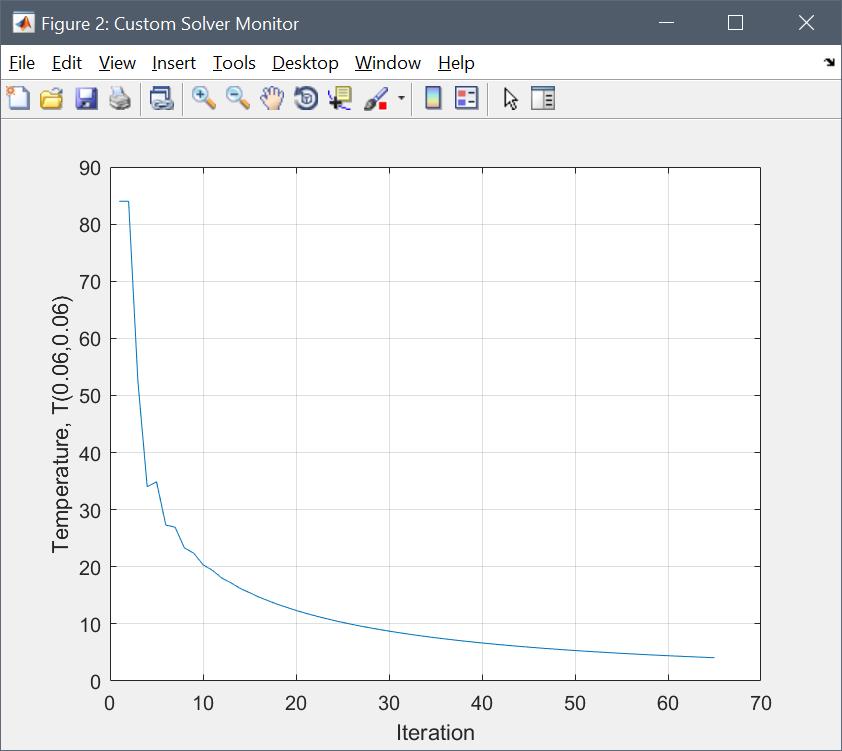
A simple use of solver hooks can be to monitor the solution process. The example below implements a function to monitor the temperature in a specific point
function [ A, f, fea ] = monitor( A, f, fea, solve_step )
persistent h_fig T
if( isempty(h_fig) )
  h_fig = figure( 'Name', 'Custom Solver Monitor' );
end
if( solve_step == 1 )
  return
end

T = [ T, evalexpr( 'T', [0.06;0.06], fea ) ];

clf
plot( 1:length(T), T )
grid on
xlabel( 'Iteration' )
ylabel( 'Temperature, T(0.06,0.06)' )
drawnow
To see it in action, save the function in a file named monitor.m, then enter the function name monitor in the Solver Hooks dialog box, and run the Shrink Fitting of an Assembly model example.
For other examples of using solver hooks see the following MATLAB m-file script examples
It is also possible to define custom solver monitoring functions by creating a m-script function with the name fea_solve_monitor.m. If present and detected by MATLAB the function will be called by the built-in solvers after each iteration or time-step with the following function signatures
function [ halt ] = fea_solve_monitor( fea, it )      % for solvestat
function [ halt ] = fea_solve_monitor( fea, tlist )   % for solvetime
where fea is the finite element problem struct, it the non-linear iteration number, and tlist the list of time steps corresponding to the number of columns in the solution vector stored in fea.sol.u. The output argument halt is a logical scalar which indicates if the solution process should be terminated early. For example, the following function for the Shrink Fitting of an Assembly model example will monitor and plot the temperature, T, as a function of time at the point (0.06, 0.06), and stop the solution process when the temperature has reached 15 degrees or lower.
function [ halt ] = fea_solve_monitor( fea, tlist );
persistent h_fig
if( isempty(h_fig) )
  h_fig = figure( 'Name', 'Custom Solver Monitor' );
end

for i=1:length(tlist)
  T(i) = evalexpr( 'T', [0.06;0.06], fea, i );
end

clf
plot( tlist, T )
grid on
title( ['T@t = ',num2str(tlist(end))])
xlabel( 'Time [s]' )
ylabel( 'Temperature, T(0.06,0.06)' )
drawnow

if( T(end) <= 15 )
  halt = true;
else
  halt = false;
end
It can be difficult to achieve convergence for models involving complex geometries, meshes, non-linear equations, and/or tightly coupled multiphysics problems. This section includes a few tips and approaches which might be helpful in such cases.
When the linear solver fails to converge one can often encounter an error message such as
Warning: Matrix is singular to working precision or
         incorrectly scaled. Results may be inaccurate.
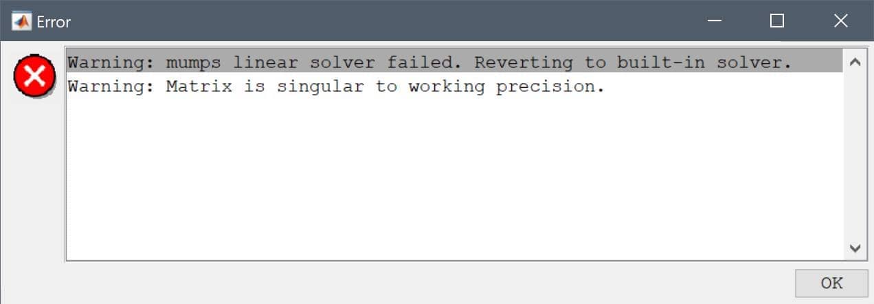
Such an error message indicates that the (finite element) system matrix the toolbox is trying to solve has failed to converge, and results in an invalid solution with "NaN" (not-a-number) entries ("NaN" entires are ignored in postprocessing and will show up as an empty plot).
This could be due to a variety of reasons, for example poor mesh quality, or invalid equations. What follows are a few things to check and consider in these situations.
A geometry including many complex features or features with very different scales (small to large, and/or thin to thick) can be difficult to mesh, or lead to poor quality meshes. In such cases it is recommended to try to simplify the geometries before meshing, such as removing small features (with the defeaturing operation) that likely will not affect the overall solution for the quantity that is of interest.
For best convergence it is desirable to have mesh elements as close to uniform as possible, meaning mesh edges and faces of roughly equal size, and also an overall small size difference as possible (large to small mesh elements). The quality of the mesh can be inspected by selecting the Grid Statistics... option from the Grid menu in the toolbox GUI (equivalent to using gridstat function the on the command line).
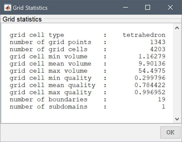
Specifically, take note of the (minimum) grid cell quality indicating how far from an ideal or perfectly uniform (quality = 1.0) mesh cell there are. And also the ratio of the minimum to maximum mesh cell volumes ideally should not be too large. If any of these ratios are very large (> 1000) it may cause convergence difficulties.
In such cases it would firstly be good to try to simplify the geometry. Secondly, try different mesh generation algorithms (such as using Gmsh instead of the Built-in algorithm) and/or setting (increasing the quality factor or smoothing steps).
Lastly, if the geometry is very thin in one specific (x, y, or z)-direction, it can sometimes help to first scale the geometry (larger) in this direction, mesh it, and then scale the mesh back. Although not yet available in the GUI, the gridgen_scale function can be used to accomplish this on the command line.
Furthermore, convergence can be difficult if equation and/or boundary coefficients and expressions are invalid, such as division by zero, or if there are large differences and jumps in coefficients between subdomains.
If logical switch expressions (involving < > =, for example T*(T>300)) are used, it might be better to try implement them as smoothed Heaviside functions to avoid discontinuous jumps as described here.
If all of the above have been explored, and the system is still difficult to solve. It can in some cases help to change the linear solver. Usually either mumps or the built-in backslash solver are the most reliable and robust linear solver options.
Finally, using external solvers (FEniCS for FEA and multiphysics and/or OpenFOAM and SU2 for CFD problems) may also be an option to try if the built-in solvers fail.
An iterative strategy such as Picard/fixed point or Newton's method is used to solve non-linear problems. First, apply the linear solver recommendations described previously. Fundamental to convergence of these methods is the initial or starting guess (initial solution). If the starting guess is too far away from the actual solution, the methods will typically not converge. Therefore ideally try to choose an initial solution as close to the expected one as possible.
The following is a list of solver settings and parameters that might be recommended for highly non-linear problems.
backslash option, which is equivalent to using the UMFPACK/SuiteSparse direct sparse linear solver.u_new = alpha * u_new + (1 - alpha * u_old)). A value between 0.5 - 0.8 can help with convergence (but also typically increases the required number of iterations).isotropic diffusion. For very highly non-linear problems higher-order artificial diffusion such as shock capturing might be better to avoid, as they make the problems even more non-linear. Moreover, for incompressible flow equations it might be better to disable pressure stabilization and instead use P2P1 finite element discretization to simplify the equations.Backward-Euler with standard Row sum lumping of the mass matrix. Moreover, smaller time steps decreases changes between the steps which also should be easier for convergence.Fluid-structure Interaction (FSI) problems feature a dedicated solver (fsisolve) which handles the physics coupling between the fluid and solid domains, and allows for movement of the grid by using a solid extension mesh motion technique with Jacobian-based stiffening [1].
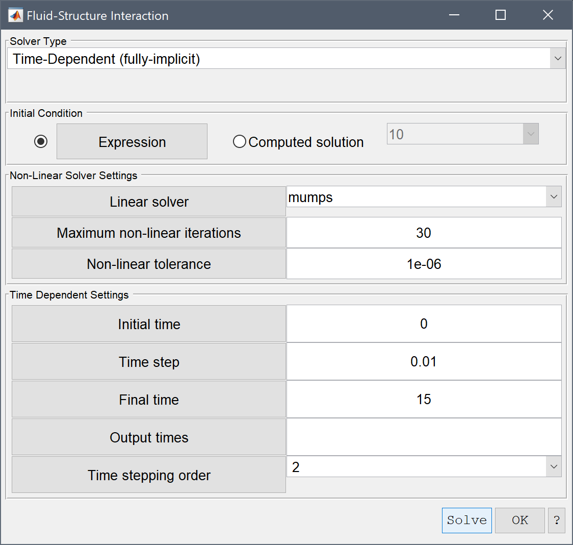
The FSI solver supports time-dependent problems with either fully-implicit or semi-implicit discretizations (with explicit geometry treatment). The Initial Condition section allows for either initial conditions from a pre-defined constant or expression, or interpolated from a previously computed solution.
The Time Dependent Settings section allows for prescribing the Initial time, Time step size, and Final time. Specific Output times can also be supplied as a vector of specific times to save and output (default [t0:tstep:tend]). Moreover, the order and accuracy of the employed time discretization schemes can also be selected (1st to 5th for the fluid domain using a Backward Difference Formula (BDF) discretization, and Newmark scheme for the solid domain).
[1] A. Quarteroni, A. Manzoni, F. Negri. Reduced Basis Methods for Partial Differential Equations. An Introduction, Springer, 2016.
The following functions can be used on the MATLAB command line interface for to solve FEATool Multiphysics simulation problems.
| Function | Description |
|---|---|
| fenics | Solve problem with the external FEniCS solver |
| fenics_data | Convert FEATool problem to FEniCS |
| openfoam | Solve problem with the external OpenFOAM solver |
| su2 | Solve problem with the external SU2 solver |
| fsisolve | Solver for fluid-structure interaction problems |
| solvelin | Wrapper around linear sparse Ax=b system solvers |
| solveeig | Solve eigenvalue/frequency problem |
| solvestat | Solve stationary problem |
| solvetime | Solve time-dependent/instationary problem |