Graphical User Interface

This section describes how to use the FEATool Graphical User Interface (GUI). Please note that the GUI may look different depending on your system configuration, FEATool and MATLAB versions.

Main GUI Window

After launching FEATool in MATLAB (by typing featool at the command prompt) the GUI will load. The main GUI window which will open is composed of the main GUI axes, top menu and toolbar, left vertical mode and tool button bars, and also command log and message windows. The functions of these GUI components are explained below.

Main GUI Axes

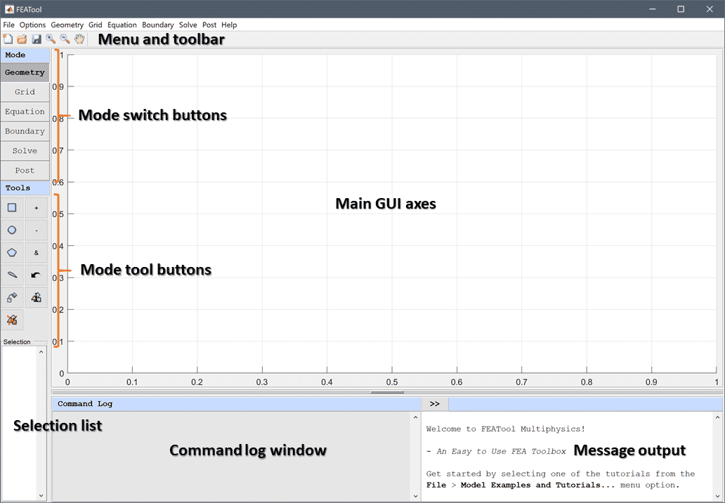
The main GUI axes is where the geometry, computational grid, and postprocessing results are displayed. The camera view can be controlled by the Zoom In , Zoom Out , Pan , and in 3D also the Rotate , XY , , XZ , YZ , Reset , and Extents view buttons in the top toolbar.

Menus

On the top of the GUI toolbar there are menus for file, options, mode, and help operations. The function of these menus are described in detail below

The File menu features the following options

• New Model... clears the old model data and opens the New Model dialog box.
• Load Model/GUI Script... allows for opening and loading a previously saved binary model (.fea file) or run a GUI script (.fes file).
• Save As Model File... allows for saving the current state of a model in binary format (.fea file).
• Save As GUI Script... allows for saving the commands used in the session as a GUI playback script files (.fes file). Note that GUI script files does not save the grids or solutions, just the sequence of GUI actions that created them.
• Save As MATLAB Script... allows for saving the commands used in the session as a MATLAB m-script model file (.m file). Note that m-script models does not save the grids or solutions, just the FEATool function calls that created them.
• Save As Python Script... allows for conversion and export of models to FEniCS Python scripts (.py file)/hdf5 mesh files (.h5 file).
• Clear/Reset Script Logs Clears the GUI and MATLAB m-script command logs.
• Create Model Report... Generate report of current modeling session in Html, PDF, Microsoft Word/PDF, Latex, or XML formats. This is equivalent to saving the model as a MATLAB script, and running the MATLAB publish command on the m-file. (Note that report generation may take some time as all geometry, mesh generation, and solution steps are repeated to capture output and images for the report.)
• Model Examples and Tutorials... Automatically runs the selected tutorial model.
• Export FEA Struct To MATLAB exports the model problem and definition struct to the main MATLAB workspace as the variable name fea.
• Exit closes and exits the FEATool GUI.

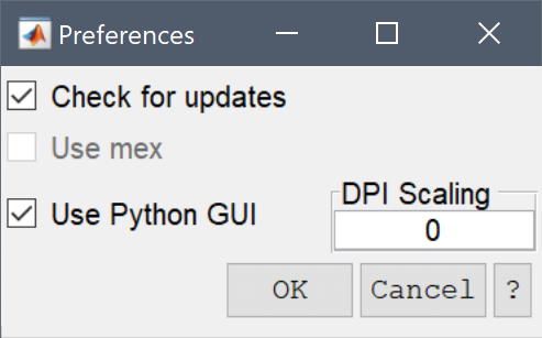
The Options menu allows the axes and grid settings to be modified (these settings are described in the axes/grid settings section below).

The Geometry menu allows for switching to Geometry Mode, creating geometry objects (Create Object), Copy/Transform Objects..., and also accessing the Combine Objects... option which allows specification of more complex formulas for geometry object composition. 3D geometries support a 2D Workplane... to be created from which planar shapes can be extruded and revolved. Geometry export and import between FEATool geometry structs, BREP, IGES, OBJ, PLY, STL, and STEP CAD formats, as well as Gmsh (geo), and Triangle (poly), and bitmap image formats (BMP, JPG, PNG, TIFF) are also supported.

The Grid menu allows for switching to Grid Mode, Converting Grid Cells between triangular and quadrilateral cells in 2D, and between tetrahedral and hexahedral cells in 3D. View Subdomains... and View Boundaries... can be used to view resulting geometric entities and their corresponding numbering. A partial selection of mesh cells can also be shown with the View Selected Cells... menu option, while viewing and modifying meshed boundaries is done using Boundary Numbering.... Lastly, the Grid Statistics... option displays relevant stats for the mesh, such as the number of grid points, cells, and quality measures.

Grid Mode also supports import and export of grids through external files (and the main MATLAB workspace), these option can also be accessed from the Grid menu

• Import Grid > From MATLAB Workspace... imports a valid FEATool grid struct from the main MATLAB workspace.
• Import Grid > FEniCS/Dolfin Format... imports a grid in FEniCS/Dolfin format (.xml file) (impexp_dolfin).
• Import Grid > FEniCS/HDF5 Format... imports a grid in FEniCS/HDF5 format (.hdf5 file) (impexp_hdf5).
• Import Grid > GiD Format... imports a grid in GiD format (.gid file) (impexp_gid).
• Import Grid > Gmsh Format... imports a grid in Gmsh format (.msh file) (impexp_gmsh).
• Import Grid > Triangle Format... imports a 2D Triangle grid (.node/.ele files) (impexp_triangle).
• Import Grid > VTK Format... imports a ParaView compatible VTK format grid (.vtk file) (impexp_vtk).

• Export Grid > To MATLAB Workspace exports a grid struct to the main MATLAB workspace with the variable name grid.
• Export Grid > FEniCS/Dolfin Format... exports a grid in FEniCS/Dolfin format (.xml file) (impexp_dolfin).
• Export Grid > FEniCS/HDF5 Format... exports a grid in FEniCS/HDF5 format (.hdf5 file) (impexp_hdf5).
• Export Grid > GiD Format... exports a grid in GiD format (.gid file) (impexp_gid).
• Export Grid > Gmsh Format... exports a grid in Gmsh format (.msh file) (impexp_gmsh).
• Export Grid > OpenFOAM Format... exports a grid in OpenFOAM format (grid2foam).
• Export Grid > PLY Format... exports a 3D PLY grid file (.ply file) (export_ply).
• Export Grid > STL Format... exports a STL grid file (.stl file) (impexp_stl).
• Export Grid > Triangle Format... exports a 2D Triangle polygonal geometry description (.poly file) (impexp_triangle).
• Export Grid > VTK Format... exports a ParaView compatible VTK format grid (.vtk file) (impexp_vtk).
• Export Grid > Web Browser... exports a html plot of the grid to the web browser.

The Equation and Boundary menus allows for switching to Equation/Boundary Modes and also opening the Equation/Boundary Settings... dialog boxes (see the equation andboundary" mode sections). Moreover, the Model Constant and Expressions... option allows for input of modeling variables and expressions that can be used in equations and boundary settings, and postprocessing. Point sources and constraints can also be added here with the corresponding Point Sources... and Point Constraints... menu options. In 3D the Edge Constraints... option is also available to add constraints on boundary edges. Physics modes can be removed with the Remove physics modes... option in the equation menu. In addition Boundary Integral Constraints... and Subdomain Integral Constraints... can also be applied.

The Solve menu similarly allows for switching to Solve Mode and also opening the Solver Settings... dialog box (these settings are described in the solver settings section). This menu also features an option to Get Initial Solution which computes the expressions defined in the equation settings Initial Condition fields and returns this as the solution.

The Post menu allows for switching to Postprocessing Mode, and opening the Plot Options... dialog box (see the postprocessing settings section below). In addition there are options for evaluating the minima and maxima for general expressions with Min/Max Evaluation..., points and line evaluation Point/Line Evaluation..., and integration of postprocessing expressions over subdomains Subdomain Integration... and boundaries Boundary Integration.... Animate/Playback Solution... allows for creating animations and videos of results, while Postprocessing Settings... enables changing settings such as smoothing of gradients. Moreover, the solution and postprocessing data can also be exported to be used with the Export Results... menu option in CSV, ParaView (VTK/VTP), and Webbrowser compatible file formats.

The Help menu can be used to access the FEATool Documentation... suite, FEATool Website..., Send Feedback..., and open the About... information dialog box which shows FEATool version information. Activate FEATool... is used to activating a license, by entering a FEATool activation token which is sent to the online licensing server to generate license keys. Activated systems can be de-activated tomove the license" to a different/new system, to do this select the Release License... menu option.

Selecting System Info... menu option shows the current installed system and software components and their versions, and the Log file... of the current session can be viewed and saved by selecting the corresponding menu entry.

GUI Toolbar

The top GUI toolbar contains the following shortcut buttons (note that the GUI might show different options and icons depending on the MATLAB version used)

• New Model starts a new model definition
• Load Model loads a FEATool model
• Save Model saves the current FEATool model
• Zoom In (and Out in 3D) the main view axes
• Zoom Out the main view axes (2D)
• Pan around the main view axes
• Rotate the main view axes (3D)
• Align view with x-y plane (3D)
• Align view with x-z plane (3D)
• Align view with y-z plane (3D)
• Reset to default view (3D)
• Zoom to extents (3D)

Mode Buttons

To the left of the main view axes is the mode toolbar which consists of six mode buttons which switches between the different modes

• Switches to geometry mode
• Switches to grid generation mode
• Switches to equation/subdomain specification mode (and opens the corresponding dialog box)
• Switches to boundary settings mode (and opens the corresponding dialog box)
• Switches to solve mode
• Switches to postprocessing mode

Mode Tool Buttons

Below these buttons are the mode tool buttons which can change depending on which mode is selected.

Geometry Mode

• Creates a line geometry object (only in 1D)
• Creates a square/rectangle
• Creates a circle/ellipse
• Creates a polygon
• Creates a NACA 4-series wing profile
• Creates a block
• Creates a sphere or ellipsoid
• Creates a cylinder or cone
• Creates a polyhedron
• Creates a torus
• Join selected geometry objects
• Subtract geometry objects from the largest/first selected
• Intersection of geometry objects
• Split object(s) by cutline (2D) or cutplane (3D)
• Apply chamfer/straight bevels to object(s)
• Apply fillet/rounded bevels to object(s)
• Extrude face to 3D solid
• Revolve face to 3D solid
• Loft faces to 3D solid
• Undo/revert composite or transformed geometry object
• Copy and/or transform (move, scale, and rotate) selected geometry object
• Delete selected geometry objects
• Inspect/edit properties of selected geometry object

Grid Mode

In grid mode the overall global maximum grid cell size variable hmax can be changed with the Grid Size edit field and slider in the grid tools toolbar.

• Initialize an unstructured grid
• Uniform grid refinement
• Advanced grid settings and grid generation algorithm selection

Equation Mode

• Open the equation settings dialog box
• Opens the constants and expressions dialog box
• Set point source terms/loads
• Define integral constraints over subdomains

Boundary Mode

• Open the boundary settings dialog box
• Set point constraints (Dirichlet)
• Define integral constraints over boundaries
• Define edge constraints (only in 3D, Dirichlet)

Solve Mode

• Solve problem with initial conditions as prescribed in the solver settings
• Solve problem with last solution as initial value
• Open solver settings dialog box
• Solve multiphysics problem FEniCS external solver
• Solve fluid flow problem with the OpenFOAM external CFD solver
• Solve fluid flow problem with the SU2 external CFD solver

Post Mode

• Open the postprocessing settings dialog box
• Open dialog box for exporting and sharing results to LinkedIn, Twitter, and jpeg/png image generation
• Export results to ParaView VTP/Glance web browser plot
• Export results to Plotly web browser plot

Command Log Window

Below the main GUI axes is the output terminal window which displays messages, and output from the local FEATool workspace such as information from grid generation and solvers. (Hold Ctrl + left click to save the command log window output.)

Message Window

The message window can display hints and tips that might be useful to your simulation. While running tutorial GUI scripts (.fes files) the modeling steps will be displayed here. (Hold Ctrl + left click to save the message window output.)

New Model Dialog Box

Pressing the New Model toolbar button or selecting New Model... from the File menu opens the New Model dialog box.

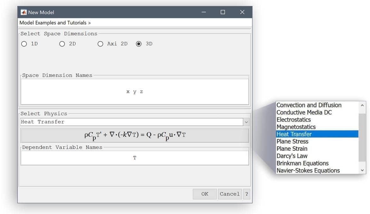
The first step in defining a new simulation model is to select the number of space dimensions to work in. The Select Space Dimensions frame allows one to choose from the 1D, 2D, Axisymmetry (for axisymmetric cylindrical coordinate systems), and 3D modeling spaces. Depending on which selection is made, the default Space Dimension Names (x, y, and z, or alternatively r and z in cylindrical coordinates) will be shown in the corresponding edit field. The space dimension variable names/labels can also be changed if desired, and are used by FEATool in defining equation, boundary, and postprocessing expressions.

The Select Physics drop down box shows a list of pre-defined physics and application modes available for the selected space dimension. By choosing one of the physics modes the corresponding physics equation and default Dependent Variable Names will be updated. This will be the first physics mode selected when defining a new model. Like the space dimension names, the dependent variable names can also be changed as long as they do not conflict with other variable names. The Custom Equation physics mode allows for any number of dependent variables to be entered. Additional physics modes can be added later by using the + tab in the Equation Settings dialog box in Subdomain Mode, as described the Multiphysics section.

To finish the initial selection process and start a new model press OK, or press Cancel to return to the previous model. Alternatively, the step-by-step tutorial models can also be started by selecting one in the top Model Examples and Tutorials... menu.

Other GUI Operations

Equation, Boundary, Solve, and Postprocessing mode usage and corresponding dialog boxes are described in the following sections.

• Physics Modes
• Solvers
• Postprocessing

Axes/Grid Settings Dialog Box

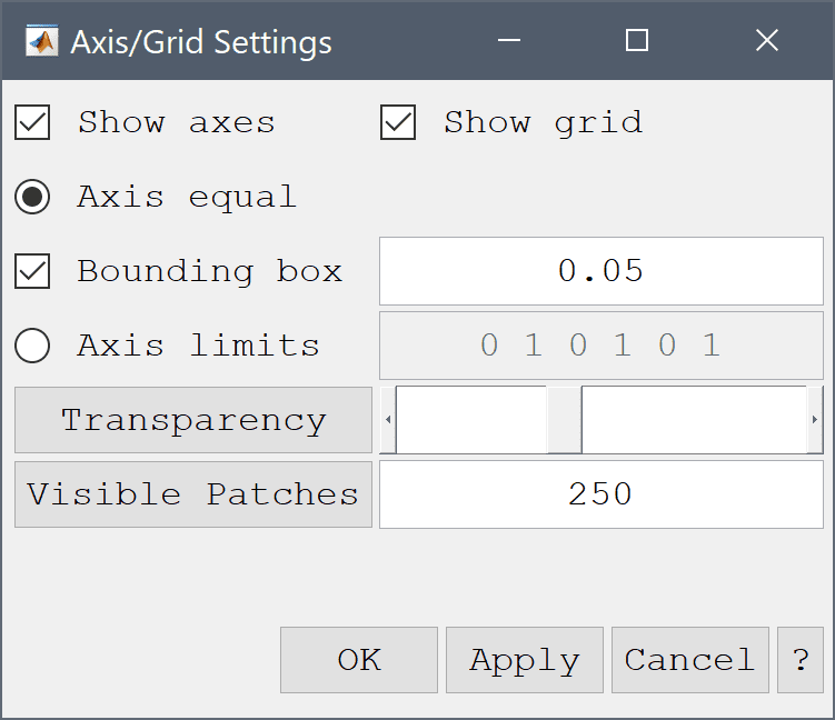
The Axis/Grid Settings dialog box features user controls for modifying the viewing plot and visualization axes. The Show axes and Show grid options can be used to show or hide the grid and axes. Axis equal enables that the axes directions have equal lengths to each other (in the x, y, and z-directions), when enabled a Bounding box can be used to add additional (relative) space with respect to the bounding box of the geometry (default 5%). Alternatively, one can also prescribe the Axis limits manually.

In 3D a slider control also allows setting of the Transparency (opacity) level of the objects. Moreover, a maximum number of Visible patches to plot when redrawing can be specified. If the total number of patches exceeds this, only the geometry outlines will be rendered during view operations (pan, zoom, rotation) in order to increase and improve potentially slow responsiveness for model with a large number of objects.

Keyboard Shortcuts

The following keyboard shortcuts are available in FEATool

• Ctrl + n Open the new model dialog box to start a new model.
• Ctrl + o Load a previously saved model file.
• Ctrl + s Open Save Model dialog box.
• Ctrl + a Select all geometry objects in geometry mode, also works in list boxes and edit fields.
• Ctrl + d Clear all selected objects.

Moreover, in 2D Geometry mode one can hold down a Shift key while using the Create circle/ellipse tool to restrict to a circular geometry instead of allowing elliptical ones.