|
|
FEATool Multiphysics
v1.18.0
Finite Element Analysis Toolbox
|
|
|
FEATool Multiphysics
v1.18.0
Finite Element Analysis Toolbox
|
The quickstart guide explains how to install and get started with FEATool Multiphysics as well as describes the modeling and simulation process. Furthermore, step by step instructions how to set up and solve five modeling examples illustrating different techniques and features of the toolbox is also included.
The FEATool Multiphysics simulation toolbox is written in the m-script language, which requires either MATLAB®, or the MATLAB® Compiler Runtime (MCR), to run and interpret the source code. MATLAB® is available from The Mathworks Inc. and the free MCR Runtime will be downloaded and installed automatically when using the stand-alone mode.
FEATool has been verified work with Microsoft Windows and Linux operating systems running MATLAB® versions 7.9 (R2009b) and later. Furthermore, a system with 4 GB or more RAM memory is recommended.
In order to use FEATool Multiphysics, the software must first be installed on the intended computer system. It is recommended to first uninstall previous versions before installing/upgrading to a newer version. Also note that, as all functionality is loaded into memory at startup, the toolbox may take some time to fully initialize and launch the GUI.
Please follow the steps below for your system to install FEATool Multiphysics as a Windows or Linux stand-alone Desktop App, or as a MATLAB® toolbox. The installers can be downloaded from the FEATool releases and installed manually, or installed as a toolbox directly from the MATLAB® APPS and Add-On Toolbar.
Follow the steps below to install the app in stand-alone mode on Windows systems (without requiring MATLAB). Note that stand-alone apps only support GUI mode, and MATLAB is required for using the script and programming API.
First download the Windows installer
Follow the steps below to install the app in stand-alone mode on Linux systems (without requiring MATLAB). Note that os requirements for Linux compatibility is Ubuntu 20.04-24.10 or Debian 12-13 (Ubuntu 25.x and later systems are not yet compatible. Note also that stand-alone apps only support GUI mode, and MATLAB is required for using the script and programming API.)
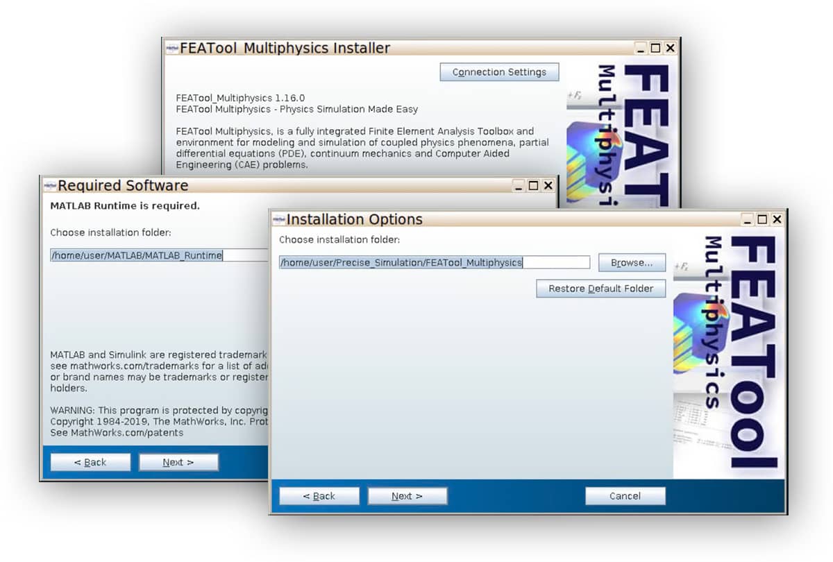
First download the Linux installer
Save it to a directory and run the installer
./FEATool_Multiphysics.install
This will first prompt for a directory to install to, for example select /home/$USER/FEATool_Multiphysics
The MCR Runtime will also need to be downloaded and installed, take note of this directory (here /home/$USER/MATLAB). Note that the runtime may require up to 2.5 GB free disk space to install.
If there are issues with the automatic MCR Runtime installation, you can download and install it manually the following link: MCR 2023a Linux Runtime (update 5)
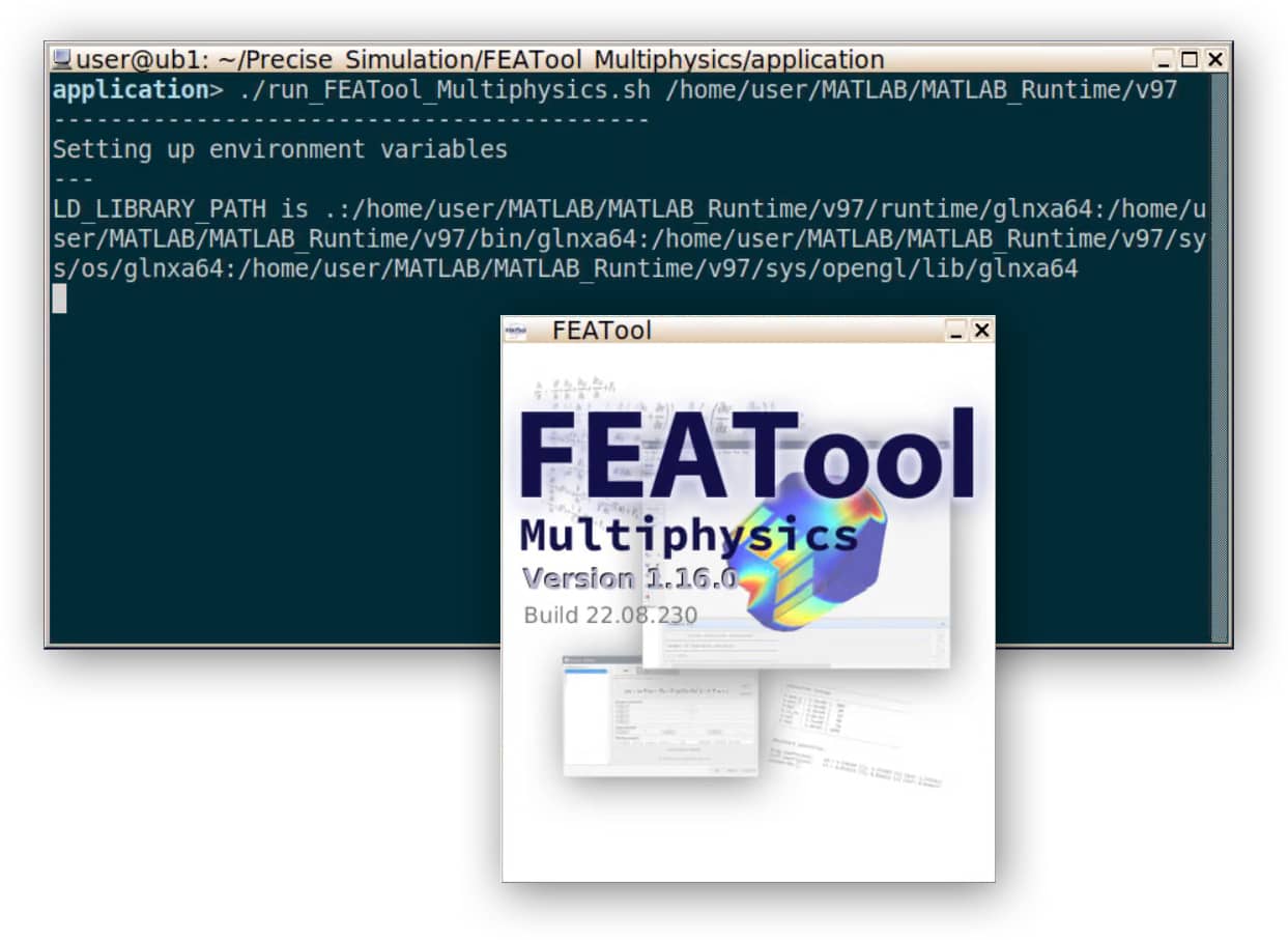
run_FEATool_Multiphysics.sh shell script from the application with the folder with the MCR runtime as input argument, for example ~/FEATool_Multiphysics/application/run_FEATool_Multiphysics.sh ~/MATLAB/R2023a
Please be patient as the application runtime can take some time to start.
MacOS is currently not available as a stand-alone App, please install FEATool as a MATLAB toolbox (Intel/x86) if you wish to use MacOS.
Follow the steps below to install FEATool as a MATLAB® Add-On toolbox (for Windows, Linux, or Intel/x86 MacOS), and to enable running MATLAB® simulation m-scripts
First download the latest FEATool_Multiphysics.mlappinstall toolbox installation file.
Press the Install button if prompted to Install to My Apps?.
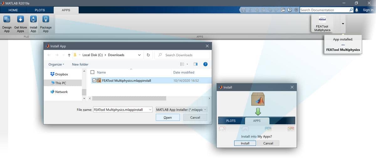
Once the toolbox has been installed, an app icon will be available in the APPS toolbar to start the FEATool Multiphysics GUI.
Note that MATLAB® may not show or give any indication of the toolbox installation progress or completion. Furthermore, using spaces and/or special characters in user and installation directory paths is not recommended as it may cause issues with the external grid generation and solver interfaces.
Although the goal is always to preserve as much backwards compatibility as possible, with the convention only to introduce significant braking changes with major version updates (for example from version 1.x to 2.0), there can sometimes be minor incompatibilities between different versions. This could for example be due to an updated geometry engine or grid generator, which can lead to slightly different meshes etc. As such one might want to keep different versions available to switch between. Although this is not possible with MATLAB® apps (as only one version can be installed at a time), one can instead store different versions in a local directory as described below. (Note that this approach is also required for using the toolbox with MATLAB® versions 2012a and earlier, which do not support MATLAB® apps.)
move FEATool_Multiphysics.mlappinstall FEATool_Multiphysics.zip
addpath(genpath('local_directory_for_version_xx'))
featool
rmpath(genpath('local_directory_for_version_xx'))
If you have purchased a license for FEATool Multiphysics, you can use an activation code or license key to activate your system.
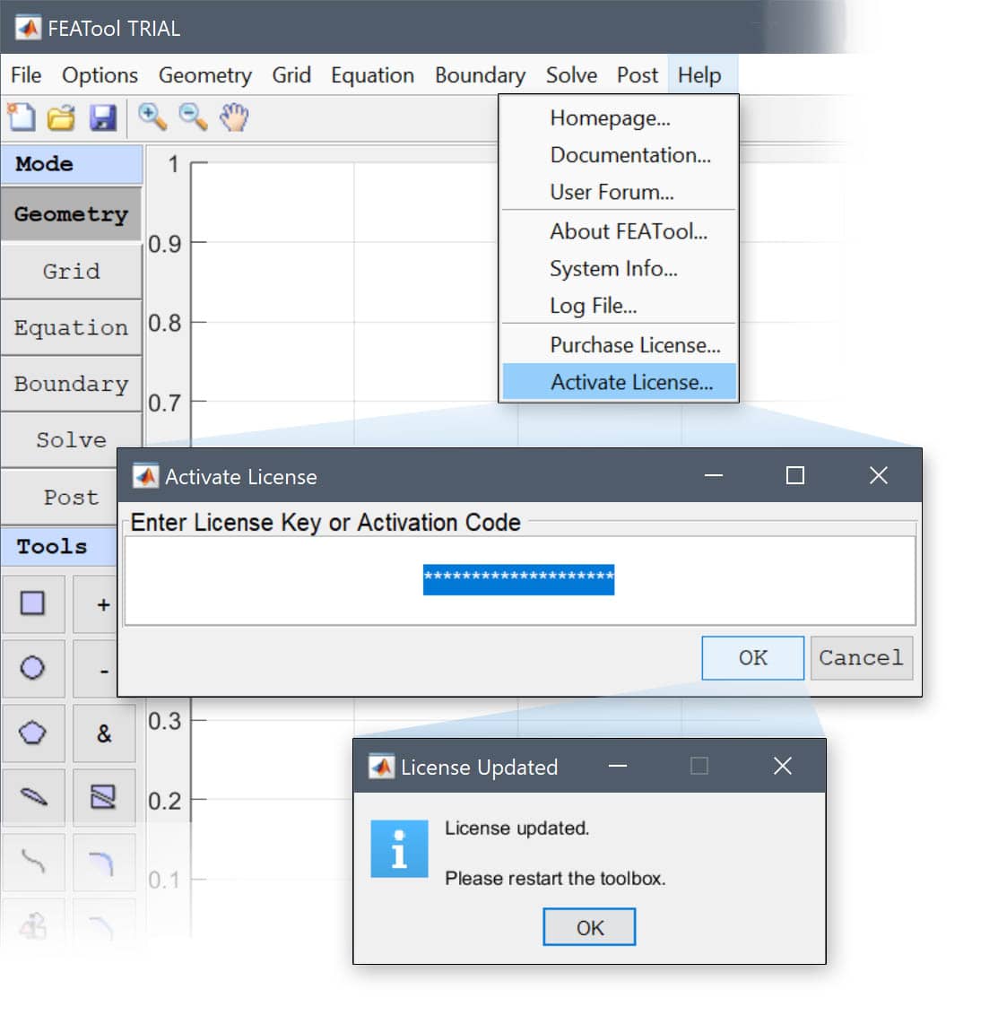
To confirm that the toolbox has been activated, restart it and select About FEATool... from the Help menu. The About dialog box will also show the license type and toolbox version information.
In the Help menu you can also open to see the System Info... and Log File..., as well as direct links to the homepage, documentation, and User Forum.
The error "Could not find matching activation code" means that the entered activation code could not be found by the license server, which may be due to either
After activation, the actual license key is stored on your computer in the file
%USERPROFILE%/Documents/MATLAB/.featool/license.dat
Please note that, licenses are in general issued per computer system/seat so that all users on the same computer/system may use the software. To allow a different user on the same computer system to use the activated license for a system one can copy the above license.dat file from the corresponding directory of the original user to the new user.
For Mac systems with ARM Mx processors it can happen that errors running executables show
zsh:1: permission denied
This usually happens if the X86 rosetta translation layer is not installed. Follow the apple guide to install it https://support.apple.com/en-us/102527.
For MacOS systems it can happen that warning dialog boxes appear and block execution with the message "executable" cannot be opened because the developer cannot be verified. In this case follow the procedure below to allow the app to run
https://support.apple.com/guide/mac-help/open-a-mac-app-from-an-unidentified-developer-mh40616/mac
The relevant executables are typically the following:
  ~/Documents/MATLAB/Add-Ons/Apps/FEAToolMultiphysics/bin/geomtool_mac
  ~/Documents/MATLAB/Add-Ons/Apps/FEAToolMultiphysics/bin/gridgen2d_mac
  ~/Documents/MATLAB/Add-Ons/Apps/FEAToolMultiphysics/bin/robust_mac
  ~/Documents/MATLAB/Add-Ons/Apps/FEAToolMultiphysics/bin/mex/assemble_f.mexmaci64
  ~/Documents/MATLAB/Add-Ons/Apps/FEAToolMultiphysics/bin/mex/assemble_m.mexmaci64
  ~/Documents/MATLAB/Add-Ons/Apps/FEAToolMultiphysics/bin/mex/assemble_s.mexmaci64
  ~/Documents/MATLAB/Add-Ons/Apps/FEAToolMultiphysics/bin/mex/assemble_se.mexmaci64
  ~/Documents/MATLAB/Add-Ons/Apps/FEAToolMultiphysics/bin/mex/earrind.mexmaci64
  ~/Documents/MATLAB/Add-Ons/Apps/FEAToolMultiphysics/bin/mex/eindarr.mexmaci64
  ~/Documents/MATLAB/Add-Ons/Apps/FEAToolMultiphysics/bin/mex/fsetup.mexmaci64
  ~/Documents/MATLAB/Add-Ons/Apps/FEAToolMultiphysics/bin/mex/fsparse.mexmaci64
  ~/Documents/MATLAB/Add-Ons/Apps/FEAToolMultiphysics/bin/mex/iluk_Cmex.mexmaci64
  ~/Documents/MATLAB/Add-Ons/Apps/FEAToolMultiphysics/bin/mex/iluk_Cmex_nosymb.mexmaci64
  ~/Documents/MATLAB/Add-Ons/Apps/FEAToolMultiphysics/bin/mex/spsetd.mexmaci64
  ~/Documents/MATLAB/Add-Ons/Apps/FEAToolMultiphysics/lib/su2/SU2_CFD_mac
If you want to de-activate and move an active license to a new computer/system, make sure your computer is connected to the internet, start the toolbox, and select Deactivate License... from the Help menu. This will deactivate, remove, and release the license from your current/old system and generate a new activation code for use with a different system (copy and store this code to activate a new system).
An optional .ini format configuration file %USERPROFILE%/Documents/MATLAB/.featool/featool.ini can be used to enable, disable, and change some toolbox settings. The available configuration options with default values are the following
    show_intro = 1
    update_check = 1
    clear_log = 1
    use_mex = 0
    linsolv = backslash
where the options
show_intro enables or disables the introduction dialog box.update_check enables or disables checking for updates on startup.clear_log clear log file on app startup.log_path optional log file path (default %USERPROFILE%/Documents/MATLAB/.featool).log_file optional log file name (default featool_log.txt).use_mex enables or disables using mex functions (mex functions potentially increase performance but can cause instabilities on some systems so is off by default).linsolv selects the default linear solver (valid options are backslash, mumps, gmres, bicgstab and amg).To verify that FEATool has been installed correctly, first starting and then closing the FEATool GUI again (this ensures that the MATLAB® paths are set up so that all FEATool functions can be found).
The FEATool installation can then be tested and validated by running simulation model and example test suites by using either of these MATLAB® commands
featool testt    % Run tests for GUI tutorials
featool teste    % Run tests for m-script examples
featool test     % Run all test suites
Please note that running the test suites may take a significant amount of time.
FEATool Multiphysics includes both GUI and CLI support for the FEniCS, OpenFOAM, and SU2 solvers. Due to very differing system and installation processes these solvers must be installed by the user separately. Please consult the corresponding FEniCS, OpenFOAM, and SU2 sections for suggested installation and usage.
FEATool Multiphysics comes with built-in support for the external mesh generators Gmsh, Gridgen2D (included with the FEATool distribution), and Triangle. External grid generators typically allows for faster and more robust grid generation, and also supports specifying different grid sizes on subdomains and boundaries. The Grid Generation Algorithm can be selected with the corresponding option in the Grid Generation Settings dialog box.
If Gmsh or Triangle is selected as grid generation algorithm and FEATool cannot find the corresponding binaries, they will automatically be downloaded, and installed when an internet connection is available. Alternatively, the mesh generator binaries can downloaded from the external grid generators repository or compiled manually and installed into any of the directories available on the MATLAB® paths (external binaries are typically placed in the bin folder of the FEATool installation directory).
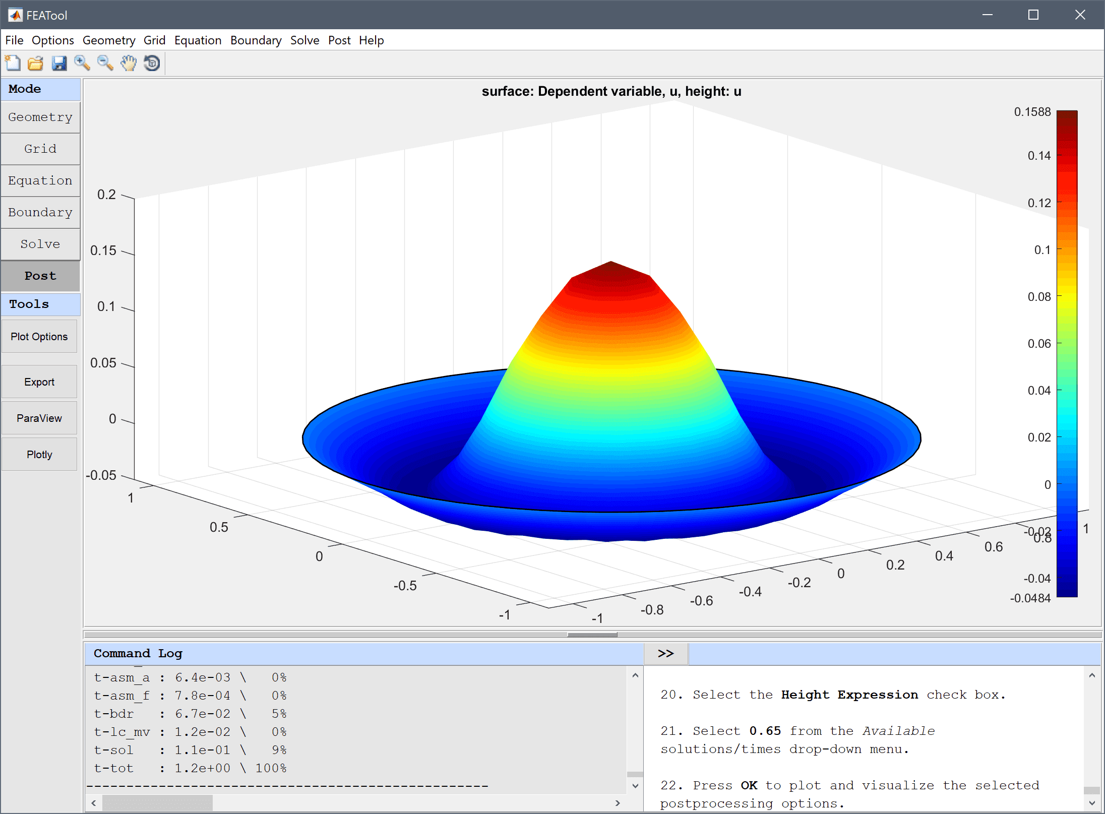
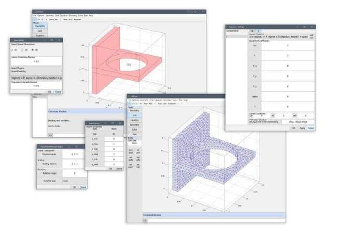
The typical modeling process in FEATool logically follows the six mode buttons located in the upper portion of the left side toolbar in the main graphical user interface (GUI) window. The modeling steps are thus as follows:
FEATool Multiphysics does not prescribe or make users use a specific unit system, it is therefore up to the user define and use consistent units. If for example a geometry length unit is chosen as meters (m), then standard SI-units are recommended for the equation and boundary coefficients. Using another length unit such as millimeters (mm) or inches, will typically require corresponding rescaling of model coefficients to preserve unit consistency.
Note however that import and export in CAD exchange formats (STEP/IGES) are assumed to be defined in meters (m), and for external external CFD solvers (OpenFOAM and SU2) SI-units are also used by default (can be changed by editing corresponding configuration files).
Pre-defined automated modeling tutorials and examples for various multi-physics applications can be selected and run from the File > Model Examples and Tutorials menu option in the GUI.
Example script files and simulation models are also available in the examples folder of the FEATool program directory. Moreover, new tutorials and articles are periodically published on the FEATool Technical Articles Blog
Five quickstart tutorials illustrate how to set up, define, and solve typical models with the toolbox are referenced in the quickstart introduction.
FEATool Multiphysics is unique in that it allows several different ways for users to work with FEM modeling and simulation. The whole spectrum from using the high-level graphical user interface down to low-level access of the fundamental matrices of the underlying finite element FEM discretization is possible. On top of this, since FEATool is written in m-script code, it can be extended and combined with MATLAB toolboxes and custom m-file scripts and functions. The four different ways of working with FEATool are using
where the last three approaches involve leaving the GUI behind in favor of the MATLAB command line and m-script files.
Designed with ease of use in mind, the graphical user interface or GUI is usually the first way one works with FEATool.
Although simple in nature, the FEATool GUI allows for some powerful features that can be utilized to extend code functionality. Every action taken in the GUI is recorded and can either saved as a Finite Element Script (fes) which can later be replayed in the GUI and is very suitable for creating tutorials. Alternatively the modeling process can be exported as standard MATLAB m-script text files suitable for command line use.
It is also possible to import and export data and variables between the GUI and MATLAB main command line workspaces by using the corresponding Import and Export menu options under the File menu.
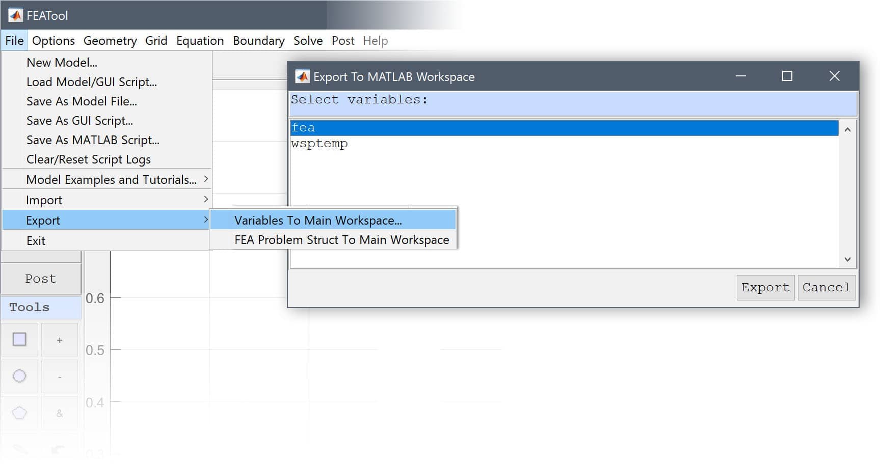
For example, the variable fea contains the FEATool finite element data struct for the current model. For example, try exporting it to MATLAB (by using the File > Export FEA Struct to MATLAB menu option) and entering the command fea to see what the fea struct contains. More information about the composition of the fea struct can be found in the problem definition section.
The first step in working with MATLAB command line and m-script FEATool models is generally to use the pre-defined physics modes. A good way to understand and learn how FEATool script models are built up and constructed is to use the Save As M-Script Model... option instead of the binary (fea) model format file.
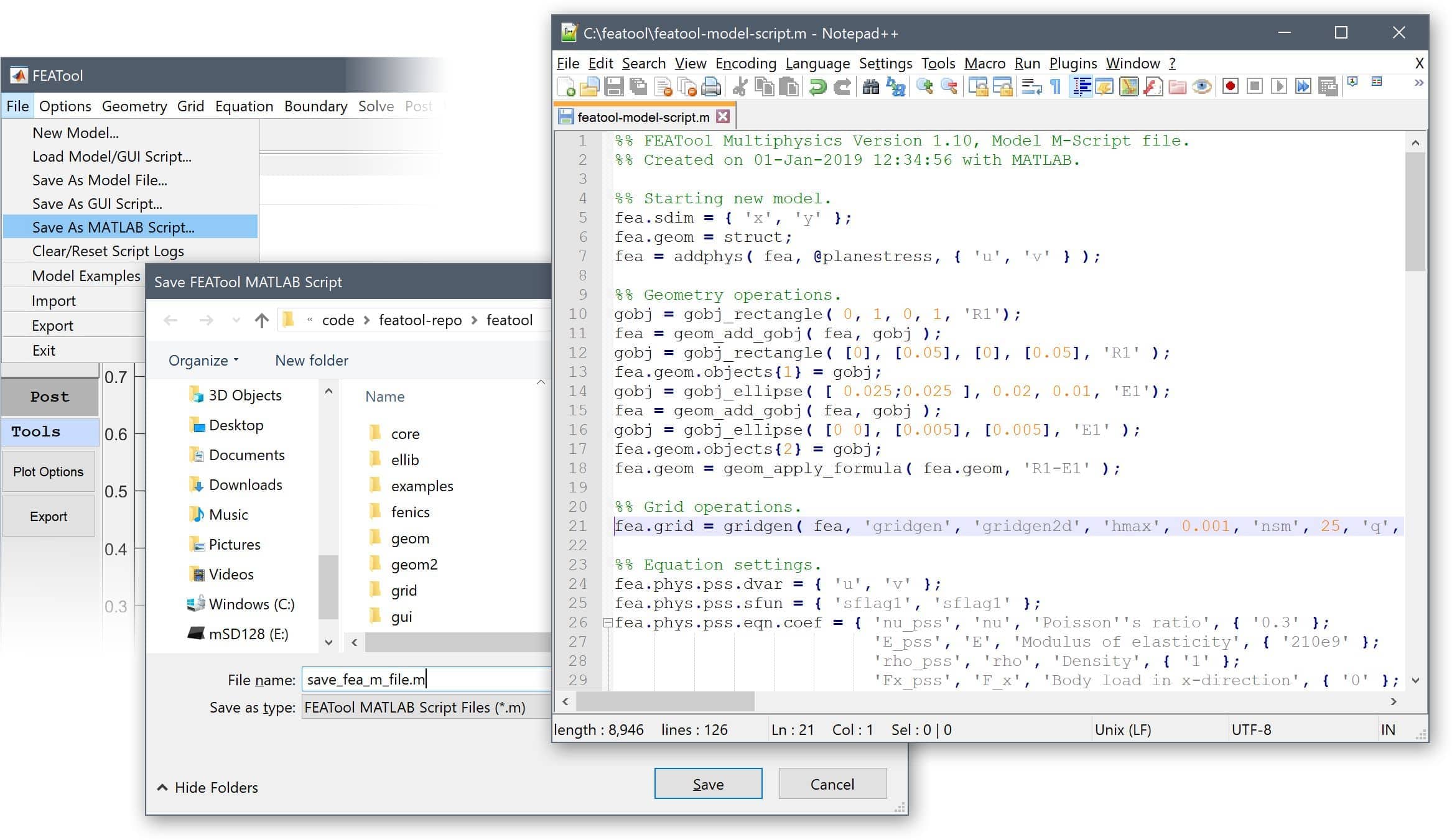
The output MATLAB m-script model source files can be opened in any text editor and the shown output corresponds directly with how the model was constructed in the GUI. Everything from the geometry definition, to solving and postprocessing has corresponding MATLAB function commands.
An example of solving the Poisson equation for a unit line defined with the Poisson physics mode can be found as the CLI Tutorial Using Physics Modes tutorial example. As can be seen in the example code, the physics modes are stored in the fea.phys field of the fea model definition struct. The actual strong PDE formulation is defined in the seqn sub-field, in this case
fea = addphys( fea, @poisson );
fea.phys.poi.eqn.seqn = 'dts_poi*u' - d_poi*(ux_x + uy_y) = f_poi'
PDE equation coefficients can be specified as
fea.phys.poi.eqn.coef = { 'dts_poi' [] [] { 1 } ;
                          'd_poi'   [] [] { 1 } ;
                          'f_poi'   [] [] { 1 } ;
                          'u0_poi'  [] [] { 0 } };
where u0_poi is the initial condition for the dependent variable u as defined in fea.phys.poi.dvar. Similarly Dirichlet and Neumann boundary conditions can be prescribed through the bcr_poi and bcg_poi coefficients, respectively
fea.phys.poi.bdr.sel  = 1;
fea.phys.poi.bdr.coef = ...
 { 'bcr_poi' [] [] [] [] [] { 0 } ;
   'bcg_poi' [] [] [] [] [] { 1 } };
Lastly, the command parsephys
fea = parsephys( fea );
parses the equations in all the fea.phys structs and enters the corresponding weak finite element formulations into the global fea.eqn and fea.bdr multiphysics fields.
If one prefers to directly work with the FEM weak formulations this is also possible as shown in the CLI Tutorial Without Physics Modes example for the same Poisson problem as above. Note how there is no phys field or call to parsephys necessary when directly prescribing the fea.eqn and fea.bdr fields
fea.eqn.a.form = { [2 3; 2 3] };
fea.eqn.a.coef = { [1 1] };
fea.eqn.f.form = { 1 };
fea.eqn.f.coef = { 1 };

n_bdr          = max(fea.grid.b(3,:));
fea.bdr.d      = cell(1,n_bdr);
[fea.bdr.d{:}] = deal(0);
fea.bdr.n      = cell(1,n_bdr);
Finally, for advanced FEM users it is entirely possible to use the core finite element assembly routines assemblea and assemblef to assemble the system matrix and right hand side/load vector after which they can be directly manipulated. Again, the corresponding Poisson problem example is described in the Poisson equation CLI tutorials. The source code for the matrix and source term vector assembly looks like the following
form  = [2 3;2 3];
sfun  = {'sflag1';'sflag1'};
coef  = [1 1];
i_cub = 3;   % Numerical quadrature rule to use.

[vRowInds,vColInds,vAvals,n_rows,n_cols] = ...
     assemblea( form, sfun, coef, i_cub,  ...
       fea.grid.p, fea.grid.c, fea.grid.a );

A = sparse( vRowInds, vColInds, vAvals, n_rows, n_cols );


form  = [1];
sfun  = {'sflag1'};
coef  = [1];
i_cub = 3;

f = assemblef( form, sfun, coef, i_cub, ...
      fea.grid.p, fea.grid.c, fea.grid.a );
Note that here we have to directly prescribe boundary conditions to the system matrix and right hand side vector.
Altogether one can see that FEATool together with MATLAB allows for many possibilities to set up, perform, and analyze multiphysics FEM simulations.
To uninstall a MATLAB toolbox, right-click on the toolbox icon in the APPS toolbar and select the Uninstall option.
Some versions of MATLAB do not fully remove toolboxes if they have been launched in the current session. It is therefore recommended to only uninstall toolboxes in a new MATLAB session. Alternatively, one can also locate the MATLAB Add-Ons/Apps directory in the userpath folder (typically found as USERHOME/Documents/MATLAB/Add-Ons/Apps) and manually delete folders corresponding to the toolbox one wishes to remove/uninstall.
Local user data is saved in the folder USERHOME/Documents/MATLAB/.featool and can be deleted (except for the license.dat file) if a user desires to completely remove or reinstall the toolbox. Note that for licensed users the license data is stored in the file USERHOME/Documents/MATLAB/.featool/license.dat which should not be deleted if one wishes to keep the license without reactivating the system).