|
|
FEATool Multiphysics
v1.18.0
Finite Element Analysis Toolbox
|
|
|
FEATool Multiphysics
v1.18.0
Finite Element Analysis Toolbox
|
OpenFOAM® is a popular and well known open-source Computational Fluid Dynamics (CFD) solver based on the traditional Finite Volume Method (FVM) for discretization of flow variables. OpenFOAM features a wide selection of solvers for incompressible, compressible, laminar, and turbulent flow regimes, and is widely used in both in academia and industry, for example in automotive engineering applications [1,2], and in Formula 1 racing to model and optimize aerodynamics performance [3,4].
The FEATool-OpenFOAM CFD solver integration makes it easy to setup and perform advanced flow simulations with the fully integrated GUI and OpenFOAM MATLAB API. As OpenFOAM includes solvers specially designed and tuned for fluid mechanics and CFD applications, it can yield a magnitude or more speedup and memory efficiency compared to the built-in direct solvers. which allows for both significantly larger simulations and compute results faster.
Note that the OpenFOAM solver binaries are not included with the toolbox distribution and must be installed separately. See the OpenFOAM installation section below for information on how to install OpenFOAM.
The FEATool-OpenFOAM solver integration allows for models created with applicable physics mode combinations listed below (with the related OpenFOAM solver application)
To use the OpenFOAM solver for a model with these physics mode combinations, press the ![]() toolbar button in Solve Mode, instead of the default solve button. This will open the OpenFOAM solver settings and control panel show below.
toolbar button in Solve Mode, instead of the default solve button. This will open the OpenFOAM solver settings and control panel show below.
The built-in, SU2, and and FEniCS multiphysics solvers can be used for these types of problems instead. Also multiple subdomains is only supported with the conjugate heat transfer model.
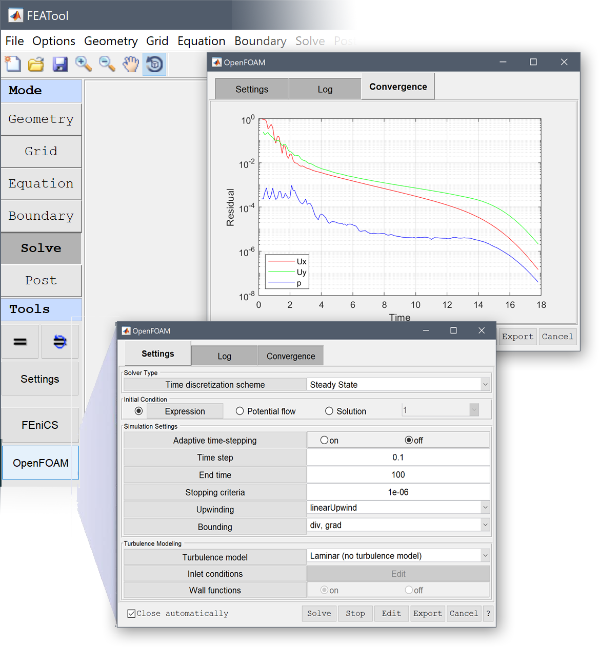
The OpenFOAM control panel and solver settings dialog box allows one to use OpenFOAM to solve CFD problems.
In the lower control button panel the Solve button will start the automatic solution process with the chosen settings. This means that the following steps are performed in sequence
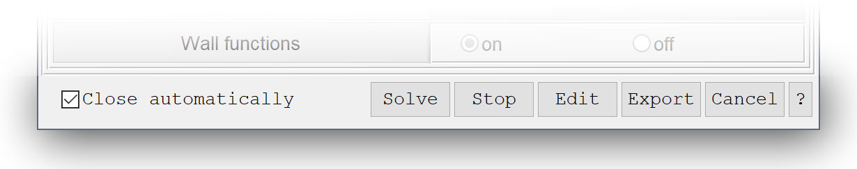
While the solution process is running the Stop button will halt/pause the solver and plot the current solution state, while the Cancel button terminates the solution process and discards the current solution (note that it can take some time for the solver register a halt event and to stop). If the Close automatically checkbox is marked, the OpenFOAM control panel will be automatically closed after the solution process has finished, and FEATool will switch to Postprocessing Mode.
During the solution process one can also switch between the Log and Convergence tabs to see and monitor the solver output log file and convergence plots in real-time. In the Convergence tab the error norm for the solution variables such as velocities, pressure, and turbulence quantities are plotted after each iteration and time step. A horizontal dashed gray line shows the convergence criteria at which point the solver will automatically stop (when reached by all solution variables). Note that for parallel simulations the convergence plots can be somewhat irregular due to the unordered log file output from parallel runs.
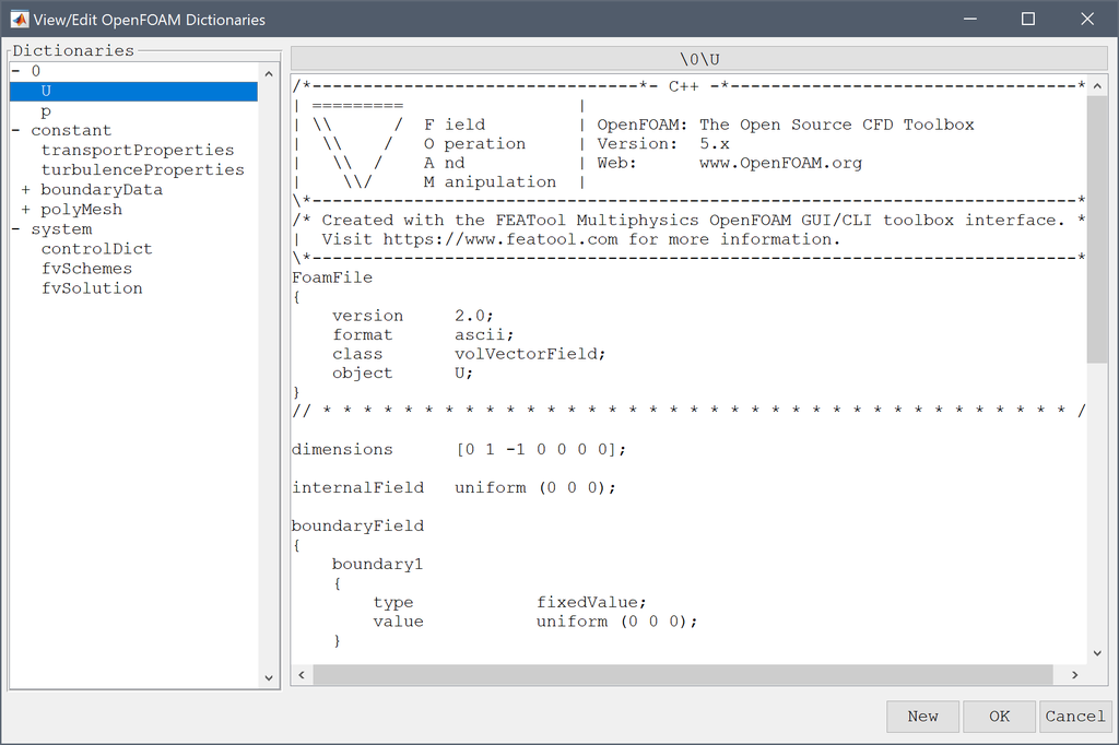
The Edit button in the control panel opens a new dialog box where OpenFOAM dictionary and case files can be viewed and edited (select the dictionary file to view/edit in the left hand side tree list). Note that manually editing OpenFOAM case files will lock the settings controls (due to potential mismatches between manual input and the dialog box controls). Open the View/Edit dialog box again and press the Cancel button to clear/reset case files unlock and re-enable GUI controls.
The Export button allows for OpenFOAM dictionary and case files to be exported for external manual processing, editing, and solving.
The following solver parameters and settings can be modified and set through the OpenFOAM dialog box and control panel.
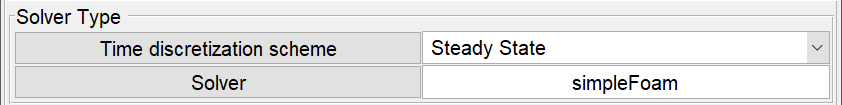
Firstly, the Time discretization scheme and main solver type can be selected according to the given problem in the drop-down box. For stationary and steady-state models the following time schemes are available
and for instationary, transient, and time-dependent problems
By default the simpleFoam OpenFOAM solver will be used for incompressible flow problems with fixed time steps and pimpleFoam if adaptive time stepping is selected. For compressible flow type problems the rhoCentralFoam or sonicFoam solver is used instead. For coupled heat transfer in a single domain (using the Boussinesq approximation) the buoyantBoussinesqSimple/PimpleFoam solver is used, while conjugate heat transfer in multiple subdomains uses the chtMultiRegion(Simple)Foam solver.
The selected OpenFOAM solver can be changed manually in the Solver edit field. Note that by manually changing the solver to an unsupported type, you must also ensure that all OpenFOAM dictionaries are defined and set up correctly for the solver to run.

Initial conditions can be specified as either constant or subdomain expressions for the solution variables using the Expression dialog box (equivalent to specifying the corresponding fields in the Subdomain Settings dialog box). Alternatively, a Potential flow solution can also be computed (with potentialFoam) and used as an initial condition, or if a previously computed Solution exists it can be used instead.
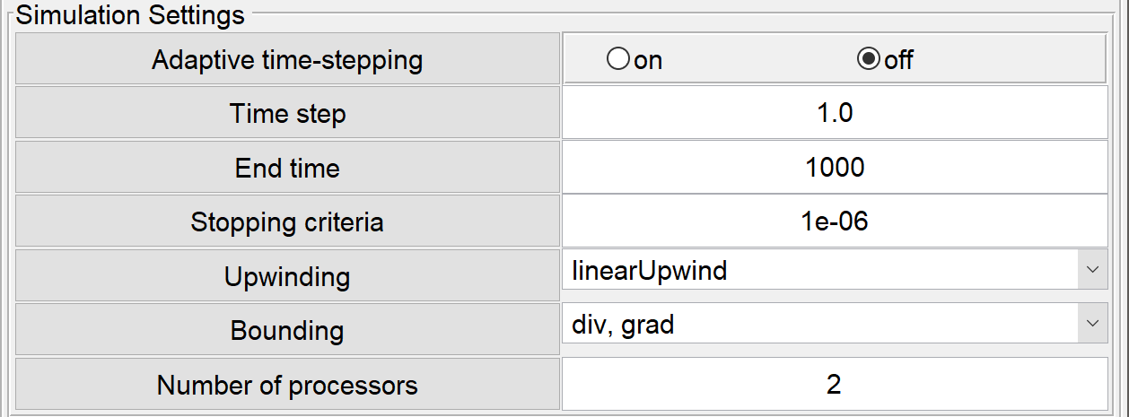
The Simulation Settings allow for specifying the following parameters
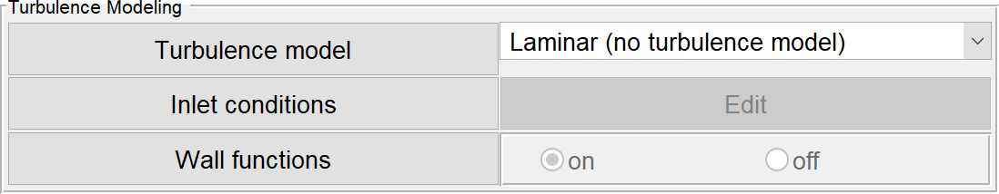
The Turbulence model drop-down box allow for the
one and two-equation RANS turbulence models to be selected (in addition to the default Laminar (no turbulence model) option).
Inlet conditions for the turbulent quantities should typically be prescribed for all inlets of the domain. One can either set the turbulence quantities directly in the turbulence inlet conditions dialog box.
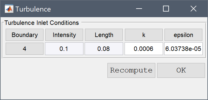
Or if not known, the turbulent quantities k and epsilon/omega can be estimated from the turbulent intensity \(I_{turb}\) (1% - 10% recommended), and \(l_{turb}\) length scale for the turbulent eddies (default 8% of the boundary length) as
\[ \begin{aligned} & k = 3/2\cdot (|\mathbf{u}|\cdot I_{turb})^2 \\ & \epsilon = C_{\mu}^{3/4}\cdot k^{3/2}/l_{turb} \\ & \omega = C_{\mu}^{-1/4}\cdot k^{1/2}/l_{turb} \end{aligned} \]
where \(C_{\mu} = 0.09\) is a turbulence modeling constant. The Recompute button will calculate the turbulent inlet quantities after changing the turbulent intensity and/or length scale.
The Wall functions setting allows for enabling and disabling standard wall functions which are typically used with meshes and grids that can not sufficiently resolve the turbulent boundary layers.
The following CFD tutorials are set up and solved with the built-in solver, but can also be solved using OpenFOAM. Simply run the tutorial, and when finished go back to Solve Mode and use the OpenFOAM solver (instead of the built-in one).
This introductory tutorial shows how to set up and solve a turbulent backwards facing step flow problem using the external OpenFOAM solver
which also can be run directly in the toolbox GUI by selecting Model Examples and Tutorials... > Fluid Dynamics > Turbulent Flow Over a Backwards Facing Step from the File menu.
A more advanced model of coupling an OpenFOAM flow field solution with a FEATool Multiphysics temperature field calculation is also available
The model can also be solved directly with OpenFOAM coupling heat transfer and fluid flow as in the m-file script model ex_heattransfer10.
The following MATLAB m-file script functions are available to setup, export, import, and process OpenFOAM data and dictionaries on the MATLAB Command Line Interface (CLI).
| Function | Description |
|---|---|
| openfoam | OpenFOAM CFD solver interface |
| openfoam_solve | Call external OpenFOAM solver |
| openfoam_data | Parse and convert fea struct OpenFOAM data options |
| openfoam_data_def_opt | Default OpenFOAM data options |
| openfoam_export | Export OpenFOAM grid and problem data |
| openfoam_import | Import OpenFOAM solution data |
| openfoam_read | Read OpenFOAM dictionary (ASCII format) |
| openfoam_write | Write OpenFOAM dictionary (ASCII format) |
| grid2foam | Convert and export grid data to OpenFOAM format |
| import_foam | Import OpenFOAM field from file |
| turbulence_inletbccalc | Compute turbulence quantities for inlet boundaries |
With a valid fea finite element data and problem definition struct, the main openfoam API function is a wrapper to automate the following solution steps
A basic minimal example to set up and solve a driven cavity flow simulation problem is shown below. First we define the grid and physics
% Define mesh and space dimension names.
fea.sdim = {'x', 'y'};
fea.grid = rectgrid();

% Add physics mode.
fea = addphys( fea, @navierstokes );

% Set x-velocity to 1 on top boundary (number 3).
fea.phys.ns.bdr.sel(3) = 2;
fea.phys.ns.bdr.coef{2,end}{1,3} = 1;

% Parse problem and set defaults.
fea = parsephys( fea );
fea = parseprob( fea );
The defined flow problem now can be solved with the built-in solver as per usual
fea.sol.u = solvestat( fea );
postplot( fea, 'surfexpr', 'sqrt(u^2+v^2)' )
Instead of using the built-in solver, we can here use OpenFOAM with the corresponding automated openfoam solver API function
fea.sol.u = openfoam( fea );
postplot( fea, 'surfexpr', 'sqrt(u^2+v^2)' )
or equivalently, manually using the functions from the steps defined above
% Define local path for OpenFOAM case files, located in
% the foam_case subdirectory of the system TEMP folder.
casedir = fullfile( tempdir(), 'foam_case' );

% Generate OpenFOAM solver options struct.
opt = openfoam_data( fea, 'casedir', casedir );

% Export mesh and dictionaries to casedir.
openfoam_export( fea, opt );

% Run OpenFOAM solver in casedir.
openfoam_solve( 'casedir', casedir );

% Import solution dictionaries.
fea.sol.u = openfoam_import( fea, 'casedir', casedir );
postplot( fea, 'surfexpr', 'sqrt(u^2+v^2)' )
The openfoam function can be used instead of solvestat and solvetime functions to solve CFD problems with OpenFOAM on the MATLAB Command Line Interface (CLI). The following is an example of laminar steady flow in a channel solved with OpenFOAM
rho = 1; miu = 1e-3; uin = 2/3*0.3;

fea.sdim = {'x', 'y'};
fea.geom.objects = {gobj_rectangle(0, 2.5, 0, 0.5)};
fea.grid = rectgrid( 50, 10, [0,2.5; 0,0.5] );

fea = addphys(fea,@navierstokes);
fea.phys.ns.eqn.coef{1,end} = {rho};
fea.phys.ns.eqn.coef{2,end} = {miu};
fea.phys.ns.eqn.coef{5,end} = {uin};
fea.phys.ns.bdr.sel(2) = 4;
fea.phys.ns.bdr.sel(4) = 2;
fea.phys.ns.bdr.coef{2,end}{1,4} = uin;

fea = parsephys(fea);
fea = parseprob(fea);

fea.sol.u = openfoam(fea);

subplot(2,1,1)
postplot(fea, 'surfexpr', 'p', 'isoexpr', 'sqrt(u^2+v^2)', 'arrowexpr', {'u', 'v'})

subplot(2,1,2), hold on, grid on
xlabel('Velocity profile at outlet'), ylabel('y')
x = 2.5*ones(1, 100);
y = linspace(0, 0.5, 100);
U_ref = 6*uin*(2*y.*(1-2*y))./1^2;
U = evalexpr('sqrt(u^2+v^2)', [x;y], fea);
plot(U_ref, y, 'r--', 'linewidth', 3)
plot(U, y, 'b-', 'linewidth', 2.5)
legend('Analytic solution', 'Computed solution')
The model parameters used here are taken from the ex_navierstokes1 example script model. The examples listed in the OpenFOAMm-file script" section similarly allow for using the OpenFOAM solver instead of the default solver. Furthermore, the openfoam function can also be embedded in user-defined custom m-scripts, which can use all other MATLAB functions and toolboxes.
An example showing how to setup an axisymmetric flow problem with turbulence and solve it with OpenFOAM on the MATLAB Command Line Interface (CLI) while displaying convergence plots in a window (using the 'control', true solver arguments).
Re = 1e5; rho = 1; miu = 1/Re; win = 1;

fea.sdim = {'r', 'z'};
fea.geom.objects = {gobj_rectangle(0, .5, 0, 15)};
n_lev = 3;
nx = 2^(n_lev-1) * 5;
ny = 2^(n_lev-1) * 50;
px = [.5, .49, .47, .44, .4, .2, 0];
px = interp1(linspace(0,0.5,length(px)), px, linspace(0,0.5,nx));
fea.grid = rectgrid(px, ny, [0, .5; 0, 15] );

fea = addphys(fea,{@navierstokes,true});
fea.phys.ns.eqn.coef{1,end} = {rho};
fea.phys.ns.eqn.coef{2,end} = {miu};
fea.phys.ns.eqn.coef{6,end} = {win};
fea.phys.ns.bdr.sel(1) = 2;
fea.phys.ns.bdr.sel(2) = 1;
fea.phys.ns.bdr.sel(3) = 4;
fea.phys.ns.bdr.sel(4) = 5;
fea.phys.ns.bdr.coef{2,end}{2,1} = win;

fea = parsephys(fea);
fea = parseprob(fea);

turb.model = 'kEpsilon';
turb.inlet = [0.001, 0.00045];
turb.wallfcn = 1;
fea.sol.u = openfoam(fea, 'turb', turb, 'hax', axes(), 'control', true, 'nproc', 1);

figure,subplot(1,2,1)
postplot(fea, 'surfexpr', 'sqrt(u^2+w^2)', 'isoexpr', 'sqrt(u^2+w^2)', 'arrowexpr', {'u' 'w'})
axis([0, .5, 14, 15])

subplot(1,2,2), hold on, grid on
xlabel('Velocity profile at outlet'), ylabel('r')
r = linspace(0, 0.5, 100);
z = 15*ones(1, 100);
U = evalexpr('sqrt(u^2+w^2)', [r;z], fea);
plot(U, r, 'b-', 'linewidth', 2.5)
The following m-file script examples show how flow problems can be defined, set up, and solved with OpenFOAM using the described API functionality. The example script models can be found in the in the examples directory of the FEATool installation folder, and feature a 'solver', 'openfoam' input parameter which can be used to directly enable the OpenFOAM solver.
API functions to generate OpenFOAM dictionaries using data from an fea struct and parameters from an opt struct (see openfoam_data.m and openfoam_data_def_opt.m).
| Function | Description |
|---|---|
| openfoam_dict_alphat | Generate alphat dictionary |
| openfoam_dict_changeDictionaryDict | Generate changeDictionaryDict dictionary |
| openfoam_dict_collapseDict | Generate collapseDict dictionary |
| openfoam_dict_controlDict | Generate controlDict dictionary |
| openfoam_dict_epsilon | Generate epsilon dictionary |
| openfoam_dict_fvSchemes | Generate fvSchemes dictionary |
| openfoam_dict_fvSolution | Generate fvSolution dictionary |
| openfoam_dict_g | Generate g dictionary |
| openfoam_dict_k | Generate k dictionary |
| openfoam_dict_meshQualityDict | Generate meshQualityDict dictionary |
| openfoam_dict_nuTilda | Generate nuTilda dictionary |
| openfoam_dict_nut | Generate nut dictionary |
| openfoam_dict_omega | Generate omega dictionary |
| openfoam_dict_p | Generate p dictionary |
| openfoam_dict_polyMesh | Generate polyMesh dictionary |
| openfoam_dict_radiationProperties | Generate radiationProperties dictionary |
| openfoam_dict_regionProperties | Generate regionProperties dictionary |
| openfoam_dict_T | Generate T dictionary |
| openfoam_dict_thermophysicalProperties | Generate thermophysicalProperties dictionary |
| openfoam_dict_transportProperties | Generate transportProperties dictionary |
| openfoam_dict_turbulenceProperties | Generate turbulenceProperties dictionary |
| openfoam_dict_U | Generate U dictionary |
Dictionary data can be generated by calling the above functions with a given fea and/or opt data structs. For example, to generate polyMesh, controlDict, and, pressure p dictionaries
opt = openfoam_data( opt );

dict.constant.polyMesh = openfoam_dict_polyMesh( fea );
dict.system.controlDict = openfoam_dict_controlDict( opt );
dict.x000.p = openfoam_dict_p( fea, opt );
The dictionaries can then be written to disk with the function openfoam_write as
casedir = fullfile( tempdir(), 'foam_case' );
openfoam_write( casedir, dict );
As OpenFOAM dictionary fields may contain special characters that are illegal in MATLAB variable syntax, non valid characters are replaced with their hexadecimal value prefixed with x. For example # becomes x23. And a variable name starting with a non-letter char is prefixed with a null character x00. Moreover, OpenFOAM list field names are prefixed with L_.
To import OpenFOAM data to the MATLAB workspace, the low level functions openfoam_read, openfoam_import, and import_foam and can be used. For example to import a pressure solution dictionary at time 1 one could use the following command
p_1_dict = openfoam_read( 'path_to_casedir/1/p' );
the imported data will be made available in the variable p_1, with fields labeled as described in the section above. Alternatively, the import_foam function can be used to import and extract a single specific field from the dictionary, for example
p_1 = import_foam( 'path_to_casedir/1/p', 'internalField' );
Lastly, all solution data from an OpenFOAM simulation can be imported and mapped to a corresponding fea struct using the openfoam_import command
[fea.sol.u,fea.sol.tlist,fea.sol.vars] = openfoam_import( fea, 'casedir', casedir );
OpenFOAM solvers are capable of performing large scale simulations on parallel clusters, and although technically possible to use the toolbox to do this, for memory and stability reasons it is typically not advised to do this from within the MATLAB environment.
For large scale simulations it is recommended to first export a model using the export functionality of the openfoam or openfoam_export functions, or use the Export button in the OpenFOAM settings andcontrol panel" dialog box which will generate corresponding OpenFOAM case files.
With the case files one can then manually launch and run the OpenFOAM solver independently without the toolbox or MATLAB (see the OpenFOAM documentation for a full explanation how to use OpenFOAM as a stand alone solver). Alternatively, if one has created OpenFOAM casefiles for a simulation outside the toolbox, the simulation can be run and monitored in the toolbox using the openfoam_solve( 'casedir', 'path_to_my_casedir', 'control', true ) command (the control flag enables graphical tracking and logging of the simulation convergence).
Solutions can then be re-imported into the toolbox if desired (using for example the openfoam_import or openfoam_read functions) as described in the section above, or processed by other external postprocessing tools such as ParaView or VisIt.
The FEATool-OpenFOAM solver integration has been extensively tested and verified with OpenFOAM version v2406, and works by performing system calls to the OpenFOAM solver executables, specifically simpleFoam, pimpleFoam, rhoCentralFoam, potentialFoam, buoyantBoussinesqSimple/PimpleFoam, chtMultiRegionFoam, sonicFoam, collapseEdges, and decomposePar. It is therefore necessary that these binaries are installed and properly set up so they can be called from system script files (bash shell scripts on Linux and MacOS, and bat/vbs scripts on Windows).
The OpenFOAM binaries are not included with the FEATool distribution as every system and OS needs specific versions for compatibility, and they must therefore be installed separately.
For Microsoft Windows systems it is recommended to install and use the pre-compiled Native-windows/mingw OpenFOAM binaries from ESI-OpenCFD (all releases and OpenFOAM for Windows installers can be downloaded from the following link https://dl.openfoam.com/source or alternatively from https://sourceforge.net/projects/openfoam/files if the original link is down or builds are missing).
For Windows systems the OpenFOAM installation is expected to be located in the default installation location, that is in the directory
%USERPROFILE%\AppData\Roaming\ESI-OpenCFD\OpenFOAM
in a subfolder with the version number, for example labeled v2406. If OpenFOAM is installed in another directory, an environment variable named FOAM_APP can be defined with the correct location so that the solver can be found.
Note that running OpenFOAM via Docker containers or Windows subsystem for Linux (WSL) is currently not supported.
For Linux systems, please follow the installation instructions and recommended distributions available from the ESI-OpenCFD website (the latest OpenFOAM Foundation distributions >= 11 (openfoam.org) are not recommended as significant incompatible changes in solvers have been made). Pre-compiled packages are available for several Linux distributions such as Debian, Ubuntu, SUSE, RedHat etc. Alternatively, the solver binaries can also be compiled from source.
For Linux systems OpenFOAM is expected to be installed in, or have a symbolic link to, the folder /opt/openfoam. Alternatively, one can also assign the OpenFOAM installation folder location by setting the environment variable FOAM_APP.
Note that running OpenFOAM via Docker containers is not supported.
For MacOS systems it is recommended to install OpenFOAM as a precompiled App available from https://github.com/gerlero/openfoam-app. If the App is installed in the /Applications directory (for example /Applications/OpenFOAM-v2406.app) the toolbox will be able to find and start it automatically when required (mounting the app in /Volumes/OpenFOAM-v####). Note that the user is then responsible for ensuring that MPI executables (mpirun or mpiexec) are available for parallel computations. Alternatively, MATLAB (and the toolbox) can be started in an OpenFOAM session (in this case the MPI libraries are already available in the OpenFOAM session).
If a compatible App is not available then OpenFOAM needs to be compiled from source and installed in the folder /opt/openfoam. Alternatively, one can also redirect to /opt/openfoam via a symbolic link, or assign the OpenFOAM installation folder location by defining an environment variable named FOAM_APP (or using the setenv MATLAB command).
The OpenFOAM source code and compilation instructions are available from ESI-OpenCFD website (the latest OpenFOAM Foundation distributions >= 11 (openfoam.org) are not recommended as significant incompatible changes in solvers have been made).
As an alternative to compiling from source, one can also install MATLAB, FEATool, and OpenFOAM in a VMWare or VirtualBox virtual machine running Linux. Note that running OpenFOAM via Docker containers is currently not supported.
Depending on how OpenFOAM was installed, one might also have to install the Message Passing Interface (MPI) libraries separately to enable parallel computations. It is recommended to use Microsoft MPI for Windows systems, and MPICH or Open MPI for Linux and MacOS systems.
Select System Info... from the Help menu to verify that the OpenFOAM installation can be found by FEATool. This will open a dialog box with details for the current system and FEATool configuration. Find the line item labeled OpenFOAM: and verify that it points to your OpenFOAM installation folder, for example
...
OpenFOAM: C:\Users\User0\AppData\Roaming\ESI-OpenCFD\OpenFOAM\v2406
...
If possible, also make sure you can run an OpenFOAM tutorial model independently of the toolbox, for example FOAM_TUTORIALS/incompressible/simpleFoam/pitzDaily.
Further information about OpenFOAM and its usage can be found in the official User Guide, the OpenFOAM wiki, and various guides available on-line such as for example OpenFOAM Tips & Tricks.
[1] OpenCFD - List of OpenFOAM® Partners, openfoam.com, 2021.
[2] Application of Detached-Eddy Simulation for Automotive Aerodynamics Development, SAE2009-01-0333, 2009.
[3] F1 turns to AWS to develop next-gen race car, zdnet.com, December 2, 2019.
[4] Aerodynamic Simulation of a 2017 F1 Car with Open-Source CFD Code, Journal of Traffic and Transportation Engineering 6, 155-163, 2018.
"OPENFOAM® is a registered trade mark of OpenCFD Limited, producer
and distributor of the OpenFOAM software via www.openfoam.com."