|
|
FEATool Multiphysics
v1.18.1
Finite Element Analysis Toolbox
|
|
|
FEATool Multiphysics
v1.18.1
Finite Element Analysis Toolbox
|
The FEniCS and related Firedrake projects are Finite Element Analysis (FEA) computing platforms aimed at modeling continuum mechanics and solving general systems of PDEs such as found in science and engineering [1,2]. As both FEATool Multiphysics and FEniCS represent and model equations with the Finite Element Method (FEM), the FEATool-FEniCS solver integration directly translates and converts the FEATool PDE equation syntax to fully equivalent FEniCS and Python simulation scripts.
As FEniCS includes a wider variety of solvers geared towards larger scale and high performance simulations, as well as symbolic analysis and optimization of the involved equation systems, it can often be worthwhile to try to use FEniCS for simulation of large or highly nonlinear problems. In contrast to the built-in linear solvers in MATLAB, FEniCS solvers support parallel execution allowing for models to be solved fast and efficiently. FEniCS has for example been used to simulate problem sizes up to 108 grid points running on up to 512 CPUs in parallel [3].
Moreover, since equations are discretized in exactly the same way by both FEATool Multiphysics and FEniCS, the produced solutions should also be virtually identical, making it possible to use FEniCS as a second or alternative step to fully validate and verify simulation results.
Note that the FEniCS binaries are not included with the FEATool distribution as every system and OS needs specific versions for compatibility, and they must therefore be installed separately. See the installation section below for information on how to install FEniCS.
Similar to what has been done with the OpenFOAM and SU2 CFD solvers discussed in the previous sections, the FEATool-FEniCS solver integration allows for easy and convenient conversion, export, solving, and re-importing models between FEATool and FEniCS directly from the graphical user interface (GUI), as well as the MATLAB command line interface (CLI).
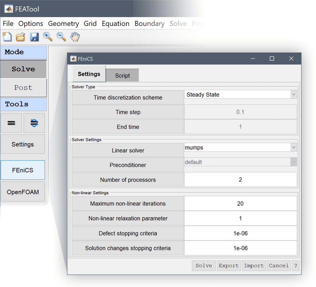
A button labeled ![]() will be available in Solve Mode toolbar for valid FEATool Multiphysics models that can be converted and solved with FEniCS. Pressing this button, instead of the default solve button, opens the FEniCS solver settings and control panel dialog box shown below. The Settings tab in the control panel is used to set and modify the solver parameters, while the Script tab will show the equivalent FEniCS Python simulation script.
will be available in Solve Mode toolbar for valid FEATool Multiphysics models that can be converted and solved with FEniCS. Pressing this button, instead of the default solve button, opens the FEniCS solver settings and control panel dialog box shown below. The Settings tab in the control panel is used to set and modify the solver parameters, while the Script tab will show the equivalent FEniCS Python simulation script.
The lower control panel buttons are used to call the FEniCS solver and control the solution process. The following functions are available:
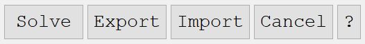
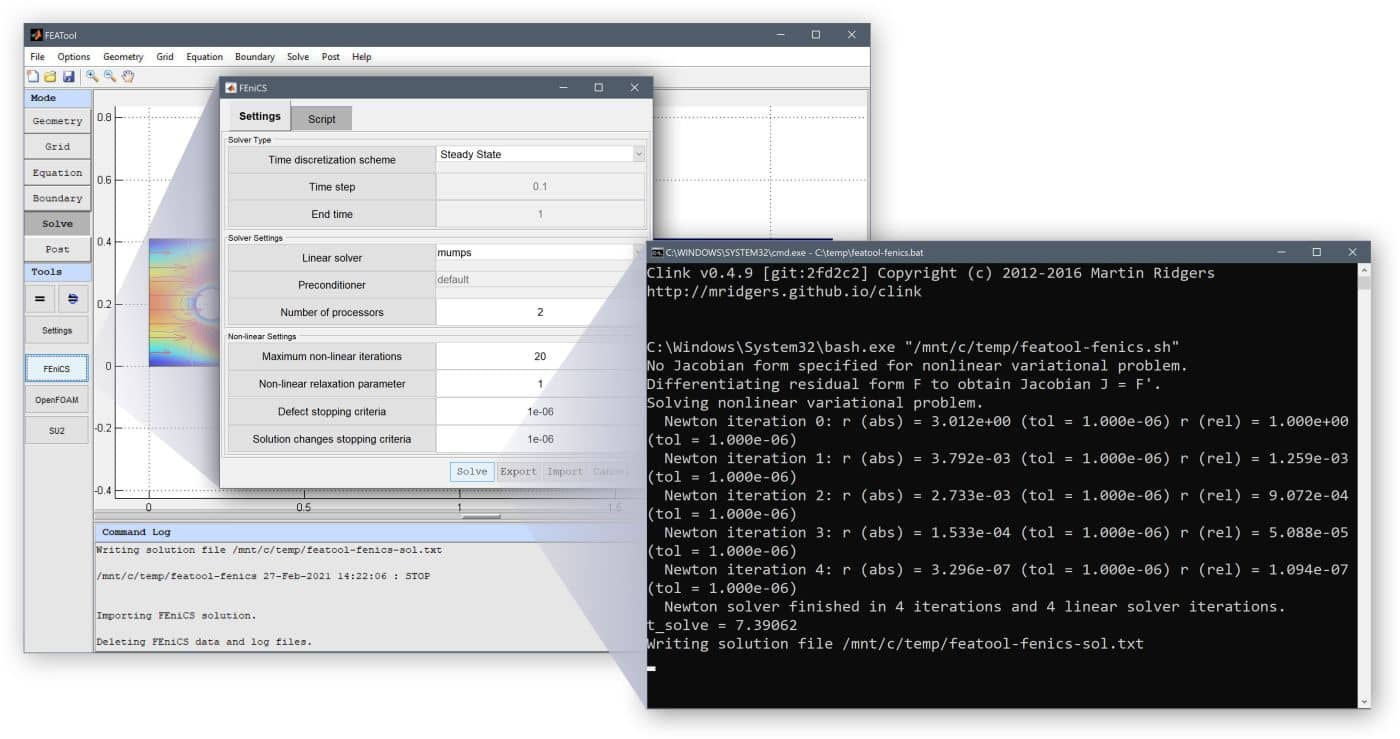
Solve executes an external system/subprocess call to the FEniCS solver and opens a terminal window showing the solution process and log. After the solution process has been completed the computed solution will automatically be imported back into the FEATool GUI (after which the control panel will be closed and FEATool will switch to Postprocessing mode and visualize the solution).
Export is used to manually export compatible FEniCS Python script and mesh files (in FEniCS HDF5 mesh format).
Import manually interpolates and imports computed solutions back into the FEATool GUI for postprocessing and visualization.
Cancel closes the FEniCS solver settings and control panel.
The ? button opens the FEniCS solver documentation section in the default web browser.
In the first section of the FEniCS solver Settings tab, Solver Type, one can select between Steady State for stationary/static simulation types, and the Backward Euler and Crank-Nicolson 1st and 2nd order implicit Time-discretization schemes for instationary simulations. When a instationary scheme has been selected the corresponding Time step size and End time parameters are enabled so that they also can be set.
In the Solver Settings section one can select the Linear solver. Depending on the installed FEniCS components one can select between the default direct linear solver (typically PETSc), mumps, or the iterative gmres, and bicgstab solvers. When using an iterative solver one can also select between the default, amg, and ilu Preconditioners. Lastly one can also select the Number of processors to use for running the computations in parallel (defaults to the number of CPU cores/2).
Lastly, in the Non-linear Settings section one can set the maximum number of (non-linear) iterations and non-linear relaxation parameter (fraction of the new to old solution to weigh in to the next non-linear iteration). The non-linear solver will terminate and stop when both the defect stopping criteria and solution changes stopping criteria are met.
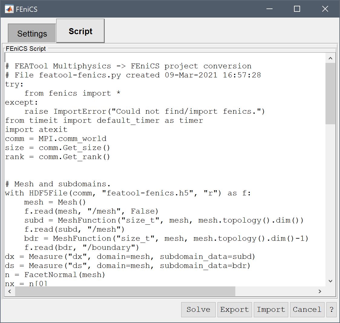
The resulting Python code from converting a FEATool Multiphysics model to FEniCS syntax can be seen in the Script tab. The script can be inspected and also manually edited to further customize and fine tune simulations. (The script shows the actual simulation script that will be executed when the Solve button is pressed, if the script is edited the edited script will be run.)
The fenics function can also be used on the MATLAB command line (CLI) and in m-file scripts to programmatically export, solve, and import with FEniCS. The following is an example to set up a simple heat transfer model on a unit circle with constant heat source term and T=0 fixed temperature on all the boundaries. In the MATLAB m-script language the model will look like the following
fea.sdim = {'x' 'y'};                % Define space dimension.
fea.grid = quad2tri(circgrid());     % Generate grid.

fea = addphys(fea, @heattransfer);   % Add default heat transfer physics mode.
fea.phys.ht.eqn.coef{6,end} = {1};   % Set unit heat source term.
fea.phys.ht.bdr.sel(:) = 1;          % Select zero temperature boundary conditions.

fea = parsephys(fea);                % Parse physics mode and fea problem.
fea = parseprob(fea);

% fea.sol.u = solvestat(fea);        % Call to default stationary solver.
fea = fenics(fea);                   % FEniCS solver call.

postplot(fea, 'surfexpr', 'T')       % Plot temperature.
Instead of the FEATool solvestat function call, the FEniCS solver is called instead with fea = fenics(fea); which automatically converts the FEATool problem defined in the fea struct and calls FEniCS to compute a solution to the problem. Note that in contrast to solvestat, the fenics function returns a modified fea struct where imported FEniCS solution will be assigned to the fea.sol.u field.
If required the fenics solver modes can be called separately (available modes are check, export, solve, and import). For example, calling the export mode
fenics(fea, 'mode', 'export', 'fname', 'featool-fenics', 'fdir', pwd);
converts the defined FEATool mesh and problem, and exports it to a FEniCS HDF5 grid file featool-fenics.h5 and FEniCS simulation script featool-fenics.py in the current working directory. The equivalent FEniCS Python FEM script for the model above is shown below
try:
    from fenics import *
except:
    raise ImportError("Could not find/import fenics.")
from timeit import default_timer as timer
import atexit
comm = MPI.comm_world
size = comm.Get_size()
rank = comm.Get_rank()


# Mesh and subdomains.
with HDF5File(comm, "featool-fenics.h5", "r") as f:
    mesh = Mesh()
    f.read(mesh, "/mesh", False)
    subd = MeshFunction("size_t", mesh, mesh.topology().dim())
    f.read(subd, "/mesh")
    bdr = MeshFunction("size_t", mesh, mesh.topology().dim()-1)
    f.read(bdr, "/boundary")
dx = Measure("dx", domain=mesh, subdomain_data=subd)
ds = Measure("ds", domain=mesh, subdomain_data=bdr)
n = FacetNormal(mesh)
nx = n[0]
ny = n[1]

# Finite element spaces.
E1 = FiniteElement("P", mesh.ufl_cell(), 1)
V = FunctionSpace(mesh, E1)

#  Function spaces.
T = TrialFunction(V)
T_t = TestFunction(V)

# Model constants and expressions.
x = Expression("x[0]", degree=1)
y = Expression("x[1]", degree=1)
h_grid = CellDiameter(mesh) if "CellDiameter" in globals() else CellSize(mesh)

rho_ht_0 = Constant(1)
cp_ht_0 = Constant(1)
k_ht_0 = Constant(1)
u_ht_0 = Constant(0)
v_ht_0 = Constant(0)
q_ht_0 = Constant(1)

# Bilinear forms.
a = ((rho_ht_0*cp_ht_0*u_ht_0)*T.dx(0)*T_t + (k_ht_0)*T.dx(0)*T_t.dx(0) + (rho_ht_0*cp_ht_0*v_ht_0)*T.dx(1)*T_t + (k_ht_0)*T.dx(1)*T_t.dx(1))*dx

# Linear forms.
f = ((q_ht_0)*T_t)*dx

# Boundary conditions.
dbc0 = DirichletBC(V, Constant(0), bdr, 0)
dbc1 = DirichletBC(V, Constant(0), bdr, 1)
dbc2 = DirichletBC(V, Constant(0), bdr, 2)
dbc3 = DirichletBC(V, Constant(0), bdr, 3)
dbc = [dbc0, dbc1, dbc2, dbc3]

# Initial conditions.
dvar = ["T"]
T_n = project(Constant(0), V)
T = Function(V)
assign(T, T_n)

# Solve.
f_data = HDF5File(comm, "featool-fenics.h5", "a")
atexit.register(lambda: f_data.close())
t_start = timer()
solve(a == f , T, dbc)
t_solve = comm.gather(timer() - t_start)
print("t_solve = %g (tot: %g)" % (max(t_solve), sum(t_solve))) if rank == 0 else None

# Output.
f_data.write(T, "/" + dvar[0])
The generated FEniCS Python script is longer and somewhat more verbose than an equivalent MATLAB m-file script since all the FEATool physics mode defaults must be expressed explicitly.
The FEniCS solution process will write the solution to the file featool-fenics.h5 which can manually be imported into FEATool with
fea = fenics(fea, 'mode', 'import', 'fname', 'featool-fenics');
or with
fea = fenics_import('featool-fenics.h5');
which also allows independently (non-FEATool) created FEniCS models and solution data to be imported into MATLAB and FEATool. The FEniCS solutions can then be postprocessed and visualized with the usual FEATool plotting and visualization functionality.
The following functions are available for working with, and converting to and from FEniCS
| Function | Description |
|---|---|
| fenics | Main FEATool-FEniCS control function |
| fenics_data | Convert and export FEATool FEA struct to a FEniCS Python script |
| fenics_import | Import and convert FEniCS HDF5 solution data to FEATool and MATLAB |
| impexp_dolfin | Import and export of mesh in Dolfin XML (ASCII) format |
| impexp_hdf5 | Import and export of mesh in FEniCS HDF5 format |
The m-script examples listed in the FEniCS tutorials section below allow for using the FEniCS solver instead of the default solver. See the fenics function listing for a full description with all available arguments and parameters.
The FEniCS solver is capable of performing large scale distributed simulations on high-performance computing (HPC) clusters, and although technically possible to use FEATool Multiphysics to do this, for memory and stability reasons it is not advised to do this from within the GUI and MATLAB.
For large and long running simulations it is recommended to export FEA models with the fenics export command or Export button in the FEniCS control panel. This will generate equivalent FEniCS Python scripts and mesh files which can be run independently, after which the solutions can be imported back into FEATool and the GUI. Furthermore, the fenics function call can also be embedded in user-defined custom m-scripts, and used with other MATLAB functions and toolboxes.
The FEATool-FEniCS integration and simulation model file export should work for general multiphysics problems using both the GUI and command line and supports most features, for example
The known subset of FEATool functionality that currently is not supported by FEniCS are
The FEATool-FEniCS solver integration has been extensively tested and verified with FEniCS version 2019.2.0, and effectively works by performing external system calls to the corresponding Python interpreter with FEniCS installed.
The FEniCS software and Python are currently not included with the FEATool distribution and must be installed separately. The FEniCS homepage and reference manual provides instructions how to install FEniCS on various systems (note that use of containers such as Docker are currently not supported).
The FEATool-FEniCS solver integration requires a Windows 10 system with the Windows Subsystem for Linux (WSL). FEniCS can then be installed in an Ubuntu or Debian WSL Linux shell by following the instructions below. Although both versions of WSL should work, it is currently recommended to use the older WSL1 due to significantly better file IO performance between Windows and Linux partitions.
For Debian and Ubuntu (WSL) Linux systems, FEniCS can be installed by opening a terminal shell and running the following commands (which automatically also installs required dependencies such as the interpreter and runtime for the Python programming language)
sudo apt-get install software-properties-common
sudo add-apt-repository ppa:fenics-packages/fenics
sudo apt-get update
sudo apt-get install --no-install-recommends fenics
For other Linux and Mac OS systems FEniCS can either be installed using the Anaconda Python environment manager, or manually compiled from source code. Note that when using Anaconda, the corresponding FEniCS environment must be activated in the MATLAB shell/session before starting MATLAB, so that FEATool can find and call the solver.
First select System Info... from the Help menu to verify that the correct Python and FEniCS installation can be found by FEATool. This will open a dialog box listing details for the current system and toolbox configuration. Find the line labeled FEniCS Version and verify that it reports the correct FEniCS version number, for example
...
FEniCS Version: 2019.2.0
...
This is equivalent to calling fenics([], 'mode', 'check') from the MATLAB command line interface.
If the FEniCS version can not be found, first verify that the FEniCS solver components have been installed and activated correctly by calling both
system('bash -c "dolfin-version"')
and
system('bash -c "python -c ''import dolfin;print(dolfin.__version__)''"')
from the MATLAB command line (python may also be aliased to python3 or python-fenics, but must start the Python interpreter with FEniCS installed). Either of these two commands should return a string with the installed FEniCS version, for example 2019.2.0.
To solve a model with FEniCS, MATLAB must also be able to make external system and bash shell calls to the specific Python environment with the FEniCS installation. Test that this works by running the MATLAB command
system('bash -c "python -c ''import fenics''"')
If any of the above checks returns an error, the Python and FEniCS installation must be corrected so that the python call command finds the installed FEniCS components.
As there can be many Python versions and environments installed on one system one must ensure that MATLAB can see the specific environment with FEniCS when calling Python. When using Anaconda Python environment this typically means one must first activate the environment in the shell used to start MATLAB (which depends on your operating system and how MATLAB is installed and started). Alternatively, one can also create an alias or symbolic link from the correct Python interpreter/installation to python-fenics. (FEATool-FEniCS solver calls will in sequence try and use Python interpreters with the aliases python-fenics, python3, and python commands.)
For Windows users with Windows Subsystem for Linux (WSL), Python and FEniCS must be installed in the default Linux distribution (if several are installed). The Windows command wsl -l will show all installed WSL distributions and the default one, and the default can be change with wsl -s DISTRO (substituting DISTRO with the name of the distribution you want to set as default).
As an alternative, one can install MATLAB, FEATool, and FEniCS in a VMWare or VirtualBox virtual machine running Ubuntu Linux.
Although not specifically illustrating use of the FEniCS solver, the majority of the tutorials available when selecting an example in the File > Model Examples and Tutorials... menu also allow for using FEniCS instead of the default solver. For example, try following the steps in the stresses in a thin plate with a hole quickstart tutorial and switch to the FEniCS solver instead of the built-in one in step 22 (solving step), and verify that it produces identical solution to the default solver.
The following m-script models, found in the examples directory of the FEATool installation folder, feature a 'solver', 'fenics' input parameter which can be used to directly enable the FEniCS solver instead of the default one
Further information about FEniCS and its usage can be found on the official FEniCS homepage and FEniCS documentation. Please use the dedicated FEniCS discussion forum for technical questions specific to the FEniCS solver if they are unrelated to MATLAB and FEATool (such as issues with FEniCS installation and modification of Python simulation scripts).
[2] Firedrake Project homepage
[3] FEniCS-HPC website - Automated solution of PDE by high performance FEM